Regular Languages Through a Haskell Lens

This lab does not involve too much programming, but is rather an opportunity for you to read some Haskell code and use it to explore some representations, constructions, and examples of regular languages. The “work” part of the lab involves a few simple exercises to make sure you understand parts of the code, a few written answers to problems (which you may nevertheless test and develop in a Haskell environment), and a couple of short coding problems.

What’s included in the module

You can find two versions of the code file on the course homepage, one a plain text file, which you can download onto your own machine and then load into hugs or ghci, and a PDF version which might be easier to read (it fits nicely on two sides of a page if you want to print it out). New! Check out the color-syntax HTML version of the Haskell source code, also below.

The two files are available as:

• RegLang.hs;
• RegLang.pdf;
• RegLang.html;

Once you have the files loaded in, you should try a few things as suggested below to get a feel for what it can do: a handful of examples are included, as well as some functions for generating test inputs. The code includes two algebraic data types, one for regular expressions (REs) and one for deterministic finite automata (DFAs).

A tour of the code (and some possibly obscure Haskell features)

Below is a quick overview of the code, in roughly top-down order. You may want to follow along as you read this section and see if you can understand what is going on. To be fair, many of you have relatively recent or relatively “stale” experience with Haskell, so I have included some tips on things that you might not remember or might not have been exposed to yet.

• RE data type: This algebraic data type should look familiar, as it is just a transliteration of the algebraic or grammatical definition we saw in lecture. Remember that the names for the constructors are (initial) uppercase and followed by the types of their arguments (also in uppercase!). The names have been chosen to be relatively “unbiased” descriptions of the symbols.
• class instances: A class instance is similar to a Java interface or an abstract algebra; it captures the idea of a type (think: set) of values that support certain operations. A class instance is what we use to specify that (or rather how) a given type supports or implements the class definition. For the RE type, we have a Show class instance which tells how REs should be printed out (here they are fully parenthesized and written as ASCII: not very pretty, but readable in your terminal and at least overt about structure). (There is no show instance given for DFAs due to their transition function: in general, Haskell will not print out functions, although we could get it to work for these simple ones. In any case, the DFAs are very easy to read in the input format used in the file.) The two helper functions pop and par are used to format binary operations (etc.) in an infix style with parentheses.
  Try printing out some of the sample REs by just entering their names (e.g., axb, baa, or swd). Can you read them and understand their structure?
• the match relation: This relation (i.e., boolean- valued function of two arguments) takes an RE and a string and tells whether the string matches or not. Thinking of it as a function from REs to string-predicates, we can think of it as giving a predicate semantics to each RE. For most of the cases this is pretty straightforward, but the last two use a combination of the (pre-defined) any function (can you figure out what it does, say using its type and perhaps Hoogle?) and a helper function part that partitions a string into two pieces in all possible ways. (Try the part function out yourself on a couple of sample strings.)

• Sample REs and back-ticked operators: Haskell has a couple of useful features for infix operators: “symbolic” operator names are infix by default, but can be referenced as prefix by enclosing them in parentheses. On the other hand, when convenient, “named” operators (like the constructor Dot) can be referenced as infix by surrounding their names in “back ticks”, found in the upper-left corner of the keyboard (note: not single quote marks!). Here I have used this feature to make the examples read a bit easier; also note the used of defined variables to make things like the literals 'a' and 'b' easier to digest. Finally, the definition of the plus operator is an example of how we can use the features of the meta-language (in this case Haskell) to get a bit of “syntactic sugar”. But if you print out an example that uses the sugar, you’ll see that it is only there in the definition, not in the actual value of the example.
• Test some samples! You can try out the match function by testing it on some of the REs given here: the names are a bit whimsical, but see if you can tell what they do by finding some sample strings that you can predict their behavior on. (Once we get to the bottom of the module we will see some utilities that help do some “wholesale” testing.)
• DFAs: The next algebraic data type is for DFAs, and again it follows our lecture definition almost exactly, differing only in that it uses a “curried” constructor (of the same name as the type) taking several arguments (rather than a 5-tuple), and in that some of the components are represented using lists rather than sets. Note the inclusion of type constraints that specify that states and symbols must support equality (the “(Eq q, Eq s) =>” part). We might also have defined our automata using separate types for the states and symbols, but this would make some of the constructions more difficult: in return, we have to pay a small price in checking these machines for validity, since they might otherwise not be well defined (this is the check function; can you see what it does?).
  One other thing to note in the data type definition: the name of the type being defined is "DFA" … but the name of the constructor for values of this type is also "DFA". This is one of a few conventions people use when a data type has only one constructor: another is touse something like "MkDFA (“make a DFA”). In either case, you can think of it like calling "new ConstructorName();" in Java.
• ZF comprehensions: The "[ … | … ]" notation is what is called a “ZF comprehension” in Haskell. It is intended to look like the similar feature in standard set theory notation; it’s meaning is also similar, but it defines a list of results (of a certain shape) based on various list generators and guards. Try these examples in a terminal to see the idea:

  • [ x^2 | x<-[1..10] ]: “the list of x squared such that x comes from one through ten”.
  • [ k*3+1 | k<-[1..10], even k ]: “the list of k times three plus one, such that k comes from one through ten and k is even”.
  • [ (x,y) | x<-"abc", y<-[1..4] ]: “the list of pairs x, y such that x comes from a-b-c and y comes from one through four”. (Note especially the ordering here!)

  If you need some help understanding this notation, which is also used in a few places below in the file, see this graphical explanation … or just ask for help!
• The foldl function: In lecture and lab we have seen the foldr function, which follows the natural structure or “grain” of a list, replacing its constructors with the parameters of the fold. The Haskell Prelude features several variations on this theme, including the foldl function used here: the difference is that foldl accumulates results from left to right rather than from right to left as foldr does … and that’s just what we need to work the transition function across a string, starting with the initial state, as the acc or “acceptance” function does. (And once we have the end state, we merely have to check if it was among the list of final states included in the definition of the DFA: that’s what elem does.)
• The “@” pattern: In the definition of the acceptance function acc, there is a use of a pattern with an @-sign prefix: this feature, read “as” allows one to name the value which matched a whole pattern, as well as naming the parts of the value that matched the pattern (with embedded variable names, in the usual way). It is used here just to make it easier to check the machine as a whole for validity: otherwise, we would have to laboriously re-construct the whole machine from its parts on the right-hand side of the clause: just m is much shorter! (And also saves a bit of time and space versus an explicit re-construction.)
• Two DFA constructions: In addition to running a DFA to see if a string is in its language (using the acc function), we can also manipulate DFAs as “objects” in and of themselves. That is to say, we can for example build new ones from old, as in the two constructions given here, namely the neg function, which returns the opposite result by simply complementing the final state set (relative to the whole), using Haskell’s set difference function (\\), or by building a machine which will compute the “simultaneous product” of two machines, relative to a specified boolean operator, using the prod function. The latter is the same idea we saw in class, but now fully realized as a function on Haskell data structures; the former could of course be simulated by simply negating the result of a run using acc, but it is nice to see that we can also do it “internally” via a machine construction.
  Note that the prod construction would be ill-defined if the alphabets of the machines did not match; also note how the ZF comprehensions make for a tidy way to describe the (roughly speaking) cartesian product of lists, and the set of all pairs of final states that satisfy the combination specified by the boolean operator parameter.
• Some sample DFAs: Next are included a couple of sample DFA machine definitions, one (called baam) which corresponds to the baa “sheep” RE, and one (called bchm) which corresponds to the bch “Beach Boy” RE (the latter is named after the starting lyrics to the popular surf song Barbara Ann by the Beach Boys).
  Note how closely the format of these definitions follows the tabular style we used on the board in lecture:
  
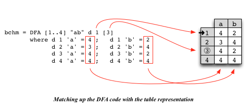
  (The semi-colons here are similar to Java’s: they simply allow us to put more than one line of code on a line of the file, thus helping the definition look more like the table.) This should make it especially easy for you to enter your own DFA definitions (see below!).
• Utility functions: This short section just contains a couple of utility functions, some of which are used in the code above, and some of which are convenient for testing purposes.

  • The cut function allows one to apply a predicate to a list of values and get a pair of lists in return, where the first half of the pair contains a list of all values for which the predicate succeeded, and the second half a list of those that failed. (Can you see how to use this to test a regular expression or a DFA on a list of possible inputs?)
  • The win function just returns the “good” or first half of a cut—this is especially helpful when the list of inputs is large, but the list of successful ones is small.
  • Finally, the lft and rgt functions just “inject” a function so that it operates on one or the other half of a pair. (These are used at a couple of points above, including in the definition of cut.)

• Generating strings over alphabet {a,b}: Finally, we have a couple of handy functions for generating test strings—these are especially useful in conjunction with cut or win from immediately above, as well as the match and acc functions. gen generates all the strings over {a,b} of a specified length (in lexicographic order, even!). abs (pronounced “ay-bees”) yields all the strings up to a given length, inclusively, ordered by length and then lexicographically. And get takes the first k strings from the same list, not by length, but just by raw number of strings, since that is sometimes more convenient.

Some things to try out

So, you’ve seen the code, and I hope you’ve tried out a few things based on the comments above, or even just exploring on your own. This section briefly describes some broader exercises you might try, followed below by some that you should be able to demo in lab. But don’t forget to just “play” with the code—you can even modify it if you like, since you can always fetch a fresh copy if you somehow manage to bollix it all up.

First off, if it wasn’t obvious from the above, you should be able to test out the match and acc functions on single and multiple examples as follows:

RegLang> match swd "abba"
True

RegLang> match swd "abbaabba"
True

RegLang> baa
(((b.a).(a.(a*)))*)

RegLang> match baa "baaa"
True

RegLang> match baa "baaaaaaa"
True

RegLang> match bch "baaaaaaa"
False

RegLang> win (match baa) (abs 6)
["","baa","baaa","baaaa","baaaaa","baabaa"]

RegLang> acc bchm "bababa"
True

RegLang> acc baam "baaaaab"
False

RegLang> win (acc bchm) (abs 8)
["ba","baba","bababa","babababa"]

Note how you use the match and acc functions just with one (other) string argument, whereas they can be partially applied and then combined with win and one of the generating functions to test many strings at once.

You can also use the constructions neg and prod to build more complex machines:

RegLang> cut (acc baam) (abs 3)
(["","baa"],["a","b","aa","ab","ba","bb","aaa","aab","aba","abb","bab","bba","bbb"])

RegLang> cut (acc (neg baam)) (abs 3)
(["a","b","aa","ab","ba","bb","aaa","aab","aba","abb","bab","bba","bbb"],["","baa"])

RegLang> win (acc baam) (abs 6)
["","baa","baaa","baaaa","baaaaa","baabaa"]

RegLang> win (acc bchm) (abs 6)
["ba","baba","bababa"]

RegLang> win (acc (prod (||) baam bchm)) (abs 6)
["","ba","baa","baaa","baba","baaaa","baaaaa","baabaa","bababa"]

Of course, you can also try out some of the utility and helper functions to make sure you understand how they work:

RegLang> part "abc"
[("","abc"),("a","bc"),("ab","c"),("abc","")]

RegLang> cut even [1..10]
([2,4,6,8,10],[1,3,5,7,9])

RegLang> get 10
["","a","b","aa","ab","ba","bb","aaa","aab","aba"]

Some things to demo!

OK, now is the time we finally get down to brass tacks: what do you need to do for credit for the lab? You should work on the following questions, producing either sample runs, definitions of examples, or even hand-written notes, for each of them. (I would in any case recommend recording your answers, whether in a file or on paper, as suitable, so that you have access during your demo.)

1. How many strings are in the list abs k as a function of k? Why?
2. Write down a regular expression which matches this informal description: strings of as and bs which have have the same letter at the beginning, somewhere in the middle, and at the end of the string (i.e., either an a or b in all 3 places), with these three occurrences separated by non-empty runs of the opposite letter (of any length > 0). Implement your design as Haskell RE called bme (for “beginning-middle-end”) and demonstrate that it works.
   As examples, all the following strings seem to meet this criterion:

   ababa   ababba abbaba   ababbba abbabba abbbaba
   babab   baabab babaab   baaabab baabaab babaaab
   

3. Design a DFA which corresponds to the previous exercise’s RE; then implement it and demonstrate that it works as intended.
4. Design a DFA which corresponds to the “Swedish rock group” example RE, i.e., the example swd in the file. (Which strings exactly does this match? How can you design the DFA? I recommend working on paper first.) Once you have the design, implement it as a Haskell DFA and show that it corresponds to the RE version, at least for {a,b} strings of length up to 8.
5. Consider the following definition of a construction which attempts to convert a machine into one which accepts the “{a,b}-opposite” by reversing the roles of the symbols in the alphabet. In other words, this opp function is trying to modify or “tweak” its argument DFA so that the new, tweaked version does exactly what the original DFA did, but with the roles of a and b swapped.

   opp (DFA qs s d q f) = DFA qs (reverse s) d q f
   

   Show that this fails to do the intended job, and explain why … but program a construction which does the job right. (Note that this {a,b}-opposite effect should in general not affect other symbols in the alphabet.)