
In a recurrent network, information is stored in two distinct ways. The activations of the units are a function of the recent history of the model, and so form a short-term memory. The weights too form a memory, as they are modified based on experience, but the timescale of the weight change is much slower than that of the activations. We call those a long-term memory. The Long Short-Term Memory model [1] is an attempt to allow the unit activations to retain important information over a much longer period of time than the 10 to 12 time steps which is the limit of RTRL or BPTT models.
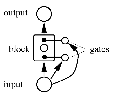
The figure below shows a maximally simple LSTM network, with a single input, a single output, and a single memory block in place of the familiar hidden unit.
 |
This figure below shows a maximally simple LSTM network, with a single input, a single output, and a single memory block in place of the familiar hidden unit. Each block has two associated gate units (details below). Each layer may, of course, have multiple units or blocks. In a typical configuration, the first layer of weights is provided from input to the blocks and gates. There are then recurrent connections from one block to other blocks and gates. Finally there are weights from the blocks to the outputs. The next figure shows the details of the memory block in more detail. |
 |
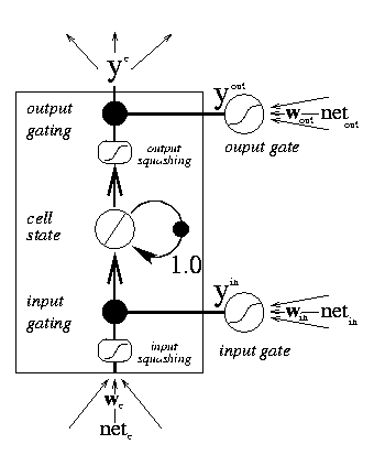
The hidden units of a conventional recurrent neural network have now been replaced by memory blocks, each of which contains one or more memory cells. At the heart of the cell is a simple linear unit with a single self-recurrent connection with weight set to 1.0. In the absence of any other input, this connection serves to preserve the cell's current state from one moment to the next. In addition to the self-recurrent connection, cells receive input from input units and other cell and gates. While the cells are responsible for maintaining information over long periods of time, the responsibility for deciding what information to store, and when to apply that information lies with an input and output gating unit, respectively. |
The input to the cell is passed through a non-linear squashing function (g(x), typically the logistic function, scaled to lie within [-2,2]), and the result is then multiplied by the output of the input gating unit. The activation of the gate ranges over [0,1], so if its activation is near zero, nothing can enter the cell. Only if the input gate is sufficiently active is the signal allowed in. Similarly, nothing emerges from the cell unless the output gate is active. As the internal cell state is maintained in a linear unit, its activation range is unbounded, and so the cell output is again squashed when it is released (h(x), typical range [-1,1]). The gates themselves are nothing more than conventional units with sigmoidal activation functions ranging over [0,1], and they each receive input from the network input units and from other cells.
Thus we have:
ycj(t) = youtj(t) h(scj(t))
scj(0) = 0, and
scj(t) = scj(t-1) + yinj(t) g(netcj(t)) for t > 0.
This division of responsibility---the input gates decide what to store, the cell stores information, and the output gate decides when that information is to be applied---has the effect that salient events can be remembered over arbitrarily long periods of time. Equipped with several such memory blocks, the network can effectively attend to events at multiple time scales.
Network training uses a combination of RTRL and BPTT, and we won't go into the details here. However, consider an error signal being passed back from the output unit. If it is allowed into the cell (as determined by the activation of the output gate), it is now trapped, and it gets passed back through the self-recurrent connection indefinitely. It can only affect the incoming weights, however, if it is allowed to pass by the input gate.
On selected problems, an LSTM network can retain information over arbitrarily long periods of time; over 1000 time steps in some cases. This gives it a significant advantage over RTRL and BPTT networks on many problems. For example, a Simple Recurrent Network can learn the Reber Grammar, but not the Embedded Reber Grammar. An RTRL network can sometimes, but not always, learn the Embedded Reber Grammar after about 100 000 training sequences. LSTM always solves the Embedded problem, usually after about 10 000 sequence presentations.
One of us is currently training LSTM networks to distinguish between different spoken languages based on speech prosody (roughly: the melody and rhythm of speech).
Hochreiter, Sepp and Schmidhuber, Juergen, (1997) "Long Short-Term Memory", Neural Computation, Vol 9 (8), pp: 1735-1780