Emerging Recursion
Jed Rembold
December 1, 2025
Announcements
- Adventure due Wednesday!
- Exam 2 corrections due end of Friday!
- Optional/Make-up Section meetings this week!
- Review materials coming out today
- Advent of Code has started!
- Can join my leaderboard using code
3198345-61d515c2 - I’ll give you some class participation points for each day’s puzzles that you complete
- Can join my leaderboard using code
- I’ll be giving you time at the end of class Friday to fill out the evaluations for this course on Canvas
- Polling: polling.jedrembold.prof
Review Question
On last Monday we looked at the selection sort, which had the following form:
def selection_sort(array):
    for lh in range(len(array)):
        rh = lh
        for i in range(lh+1, len(array)):
            if array[i] < array[rh]:
                rh = i
        array[lh], array[rh] = array[rh], array[lh]
L = [3,2,6,1]
selection_sort(L)
How many times would line 5 be reached in sorting the shown list
L?
- 4
- 6
- 10
- 16
A More Efficient Strategy
- As long as arrays are small, selection sort is perfectly workable!
- Even 10,000 elements get sorted in just over 1 second
- Less attractive to commercial applications with
huge arrays though
- Sorting a million values to take over 3 hours?!
- The \(\mathcal{O}(N^2)\) complexity
does offer a little hope though
- Sorting twice as many elements takes four times as long = BAD
- But sorting half as many elements takes only a quarter the time = GOOD!
- Can we break the array into smaller pieces and just work with those?
Recursion
A Diversion to Recursion
- Recursion is the practice of dividing a problem up into
smaller problems of the same form.
- The sub-problems must have the same form as the larger problem, or it isn’t recursion
- Since the sub-problems have the same form as the larger problem,
they can be solved using the same function
- From a code perspective, the defining characteristic of recursion is
a function which calls itself internally
- This can feel weird, but if you think about how we trace things, there isn’t anything wrong with it
- From a code perspective, the defining characteristic of recursion is
a function which calls itself internally
Solving the same (simpler) problem
- Say you needed to fundraise $1000 for an important cause
- Tough to get a single $1000 donation
- Could instead task 10 friends with raising $100
- Each friend could task 10 other friends with raising $10
- Then those friends could find 10 people who would each donate a dollar
- Solving the problem the same way each time:
- Dividing up the problem and asking those people to solve a simpler (cheaper) problem
- It must end somewhere, generally called the
base case
- Here that would have been at the $1 donation point
Recursive Factorial
The factorial function can be defined in two different ways, one of which lends itself nicely to recursion \[n! = (n-1) \times (n-2) \times (n-3) \times \cdots \times 1\] or \[n! = \begin{cases} 1 & \text{if $n$ is 0} \\ n \times (n-1)! & \text{otherwise}\end{cases}\]
The second can be expression computationally as:
def factorial(n):
    if n == 0:    # Our base case
        return 1
    else:     # Our recursive case
        return n * factorial(n - 1)
The Recursive Paradigm
Most recursive functions you encounter will have bodies that fit in the following general pattern:
if |||test for simple case|||:
    |||Compute and return simple solution without recursion|||
else:
    |||Divide the problem into one or more subproblems of the same form|||
    |||Call this same function recursively to solve those subproblems|||
    |||Return the solutions of the various subproblems|||
Finding a recursive solution is thus commonly a matter of:
- Identifying simple cases that you can solve without recursion
- Finding a recursive decomposition that breaks each problem up into smaller, simpler subproblems of the same type
Example 1: Money Raising
- Suppose we wanted to mimic the situation we described earlier, where a function needs to raise money
- Let’s print out how much each person might end up contributing
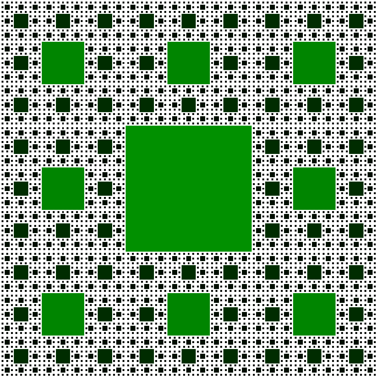
Example 2: Sierpinski Carpet
- Recursion can be visual as well!
- Many have probably seen the Sierpinski Cube in the middle of the math hearth
- How could we recreate recursively?
Merge Sort
The Merge Sort Plan
The plan with merge sort is thus to:
- Divide the array into two halves:
a1anda2 - Sort each of
a1anda2recursively - Merge elements into the original array by choosing the smallest
element from
a1ora2on each cycle
We’ll follow this process all the way through on pen and paper now to see that it works!
Merge Sort Code Implementation
def merge_sort(array):
    if len(array) > 1: #base case check
        mid = len(array) // 2
        a1 = array[:mid]
        a2 = array[mid:]
        merge_sort(a1) #recursive calls
        merge_sort(a2)
        merge(array, a1, a2)

def merge(array, a1, a2):
    n1 = len(a1)
    n2 = len(a2)
    i1 = 0 #current front indices
    i2 = 0
    for i in range(len(array)):
        if (i1 < n1 and a1[i1] < a2[i2]) or i2 == n2:
            array[i] = a1[i1]
            i1 += 1
        else:
            array[i] = a2[i2]
            i2 += 1
Merge Sort Complexity
- The work done at each level (all the work done by calls at that level) is proportional to the size of the array
- Running time is therefore proportional to \(N\) times the number of levels
So how many levels?
- Same division-by-two situation we had with Binary Search!
- Equal to the number of times you can divide the array in half until only a single element remaining
- Number of steps \(k\) was given by: \[k = \log_2(N)\]
- Total complexity of merge sort is thus \[\mathcal{O}(N \log_2(N))\]
Comparing
| \(N\) | \(N^2\) | \(N\log_2 N\) |
|---|---|---|
| 10 | 100 | 33 |
| 100 | 10,000 | 664 |
| 1,000 | 1,000,000 | 9,966 |
| 10,000 | 100,000,000 | 132,877 |
| 100,000 | 10,000,000,000 | 1,660,964 |
| 1,000,000 | 1,000,000,000,000 | 19,931,569 |
- Based on this, the merge sort would be over 50,000x faster than selection sort for an array of 1 million values!
General Complexity
Standard Complexity Classes
- Most tend to fall into one of a small number of complexity classes
| Name | Big-O | Example |
|---|---|---|
| constant | \(\mathcal{O}(1)\) | Finding the first element of an array |
| logarithmic | \(\mathcal{O}(\log N)\) | Binary search in a sorted array |
| linear | \(\mathcal{O}(N)\) | Summing over an array, or linear search |
| \(N \log N\) | \(\mathcal{O}(N\log N)\) | Merge sort |
| quadratic | \(\mathcal{O}(N^2)\) | Selection sort |
| cubic | \(\mathcal{O}(N^3)\) | Obvious algorithms for matrix multiplication |
| exponential | \(\mathcal{O}(2^N)\) | Branch and try all possibilities |
- In general, any problem whose complexity can not be expressed as a polynomial is considered intractable