Asteroid Distributions

Jed Rembold

January 26, 2026

Announcements

Homework 1
- I am working on feedback!
Homework 2
- Posted! Same partners as before (mostly)
- Due Friday night
- You’ll have everything you need after today

Recap

Kepler’s Laws
- Orbiting objects move in ellipses
  - The central object exists at one of the focus points
- Move fast when close and slow when far away
- Relationship between the period and semi-major axis
Ellipse and orbit vocabulary
Using the fitellipse libraries

Today’s Plan

Distributions
- Histograms/Density plots
- 2D variants
Asteroids
- Belt
- Resonance
- Impending doom

Visualizing Distributions

Distributions

There is a lot of stuff in space!
To understand bulk properties of objects, we commonly need to resort to looking at various distributions
Distributions can be comprised by looking at almost any variable of interest (or in some cases multiple variables)

Common usages:

EDA: exploring and bringing to light interesting properties or trends in the gathered data
By fitting mathematical expressions to the distribution, you now have a tool to use in further analysis
- This is particularly common in simulations, where simulations pull from known distributions to create physically realistic situations
- What type of mathematical distribution fits best can potentially tell you about possible inner workings that yielded that distribution
Classification: sometimes there are several distinct groupings in a distribution that can lead to various types of classification

Histograms

A histogram is a visual indication of how many times a certain variable appears
Y-axis represents counts, and the x-axis is divided into a number of bins
Data points that have a value appearing within a particular bin contribute to that bin’s count
Commonly will want to try several binning methods or sizes

Generating Histograms

Matplotlib can generate plots directly:

plt.hist( variable_list, 
          bins=num_bins )
plt.show()

Just use the hist function:

hist( variable_list, 
      breaks=num_bins )

Or, in ggplot

ggplot(data=df, 
       aes(x=variable)
      ) +
  geom_histogram()

When Bins fail

The choice of bins can often lead to distributions that might feel pretty subjective
One option is to use one of the auto-binning algorithms provided by your histogram software (read documentation)
Another, which especially makes sense for continuous data, is to look at a Kernel Density Estimate, or KDE plot
- Most common kernel is that of a Gaussian, but can be different
- Essentially stacks multiple Gaussians for each point, and then sums them together
- Results in a “smoother” looking histogram

Generating KDE Plots

Pandas can generate plots directly:
```
df[column name].plot(kind='kde')
```
- Does require scipy under the hood, so will need it installed
Can also install Seaborn and use its variants of you like
```
import seaborn as sbn
sbn.kdeplot(df[column name])
```

Just use the plot and density functions:
```
plot(density(variable_list))
```

In ggplot:

ggplot(data=df, aes(x=column)) +
  geom_density(bw='bcv')

Activity!

Here is a collection of satellite information for satellites orbiting the Earth
- It has a lot of (some nonsense) columns
- You will be interested in the column named 'Apogee (km)'
- This table originally included some satellites that are really distant from the Earth, but I’ve already filtered it a bit down to our region of interest
Create both histogram and KDE plots of the distribution of satellite apogee distances
- Can you see the outer bump formed from geosynchronous satellites?

2D Histograms and KDE Plots

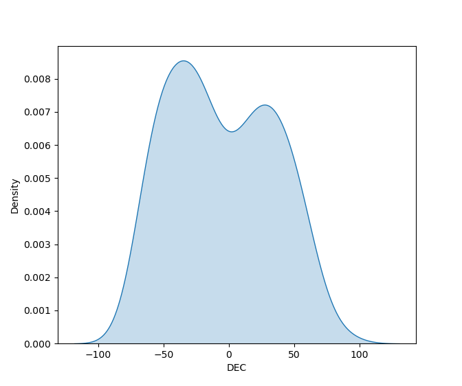
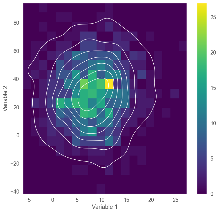
Sometimes you have multiple variables that you want to visualize together as a distribution
There are 2D analogs of both histograms and KDE plots
- One variable along each axis
- Counts or density still determine color

Multivariate Distribution Creation

Histogram in Matplotlib
```
plt.hist2d(xs, ys, bins=20)
```

KDE plot easiest through Seaborn

sbn.kdeplot(x=xs, 
            y=ys, 
            fill=True)

Histogram through ggplot

ggplot(data=df, 
       aes(x=xs, y=xs)
      ) + 
  geom_bin_2d()

KDE plot through ggplot

ggplot(data=df, 
       aes(x=xs, y=xs)
      ) + 
  geom_density_2d_filled()

Asteroid Time

Asteroids

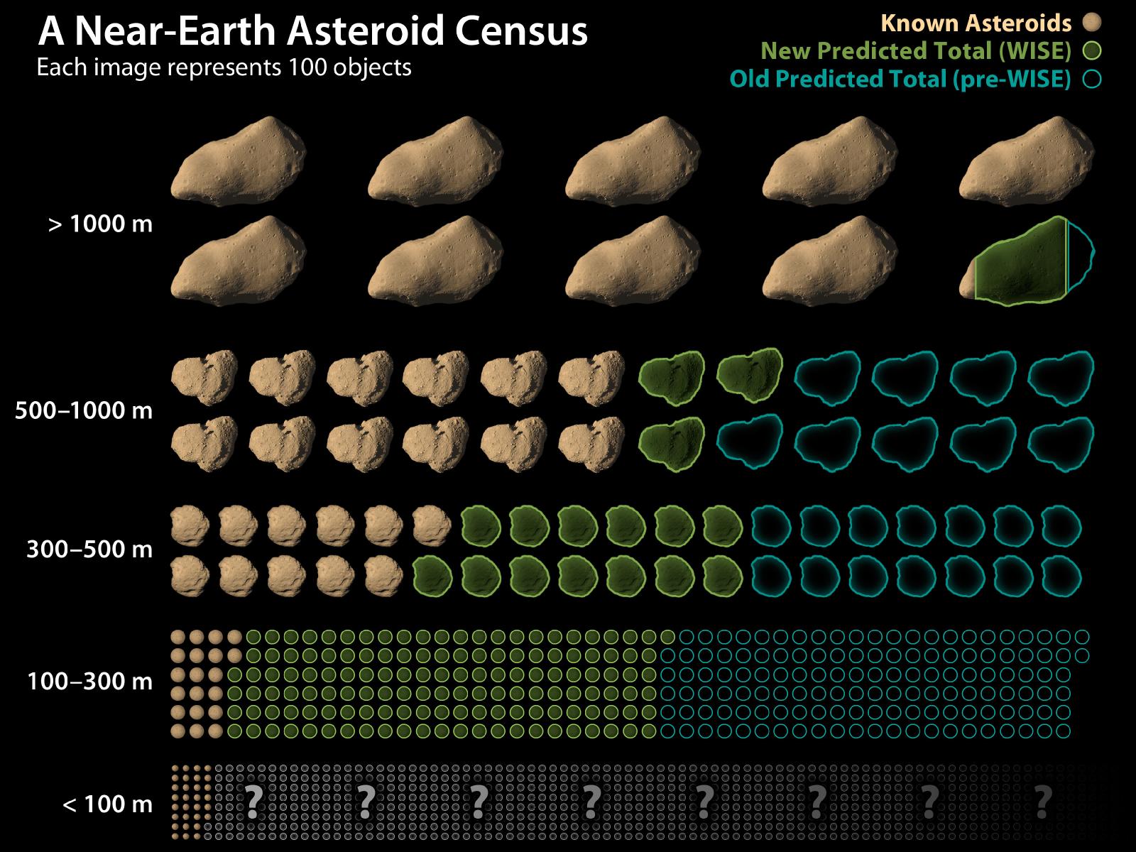
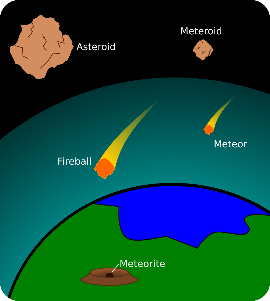
What are asteroids?

Small (relatively) chunks of rock
Maybe around a million are approximately 1 km across
- Many millions more are smaller
Irregularly shaped
Tiny = hard to see!
“Primitive”

Why a Belt?

Enough rocky material to form a body only about 3% the size of the Moon
Gravity never brought it all together, like it did for the other inner planets. Why?
- Jupiter
  - Played the role of a big bully
  - Gravity broke apart any starting planetoids before they could really get going
  - Still affects narrow bands of the belt today through orbital resonance

Orbital Resonance

When the orbits of multiple objects sync up with one being a multiple of the other, they are said to be in resonance
Resonance greatly boosts the interaction between the two bodies, with the most obvious effects on the smaller body
Imagine pushing a child on a swing:
- Pushing in rhythm with the natural swing motion works best
- Could also push every other swing, or every 3rd swing, etc
- Pushing every 1/3 swing, for instance, would be highly counterproductive

Unstable Resonance

Most often, resonances make orbits unstable
- The slow accumulation of boosts gives the smaller body more and more energy
- Generally results in the smaller body being ejected from the orbit
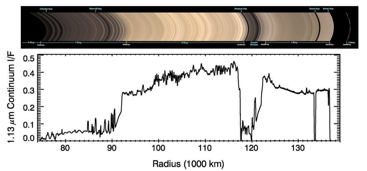
- This is the case with the Kirkwood gaps in the asteroid belt, and the Cassini division in the rings of Saturn

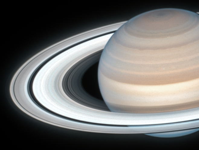
Resonance Pictured

Mimas distance from Jupiter: 186,000 km

Stable Resonance

Resonance isn’t always unstable though!
Two body resonances can be stable if the ratios / orbits are such that they prevent the objects from getting too close
Multiple orbits can influence each other to lock into a 4:2:1 resonance
- The most common is in the first three Galilean moons of Jupiter

How long before we all die horribly?

Ensuring Life

Stated goal was to find 90% of asteroids 1 km or larger with near-Earth orbits
How do we know when that goal is reached?
- Crater comparisons
- Rediscovery analysis
- Theoretical models