---
title: "Asteroids and Resonance"
author: Jed Rembold
date: January 28, 2025
slideNumber: true
theme: tokyo-night-light
highlightjs-theme: tokyo-night-light
width: 1920
height: 1080
transition: slide
---
## Announcements
:::{style='font-size:.9em'}
- Homework 1 due on Friday night!
- Example computational essay posted in Guide section
- Export each essay to a standalone HTML file, then upload the HTML file
- **Be communicating with your partners**
- Also on Friday: Virtual Alumni Career Panel for the Knight Campus Graduate Internship Program (at UO)
- Materials tracks (semiconductor, optics, polymers) at noon ([RSVP for Zoom info](https://forms.gle/coqxZoMrSN4t6Paq7))
- Bioinformatics Track at 3:15 ([RSVP for Zoom info](https://oregon.qualtrics.com/jfe/form/SV_3xeyNcG8HmNeyX4))
- Technically part of the larger Genomics in Action conference, which is free to attend if you want more than just an alumni session
- Lynde Ritzow is the recruiter for these programs, and has a long and successful history of bringing WU students into these programs. Please let me know if you have interest and would like me to make an introduction.
:::
## Recap
- Kepler's other laws
- Orbiting objects go fast when near, and slow when far apart
- Period and semi-major axis linked:
$$ \frac{a^3_{AU}}{p^2_{yr}} = \left(M_1 + M_2\right)_\odot $$
- Distributions show bulk trends
- Histograms
- KDE plots
## Today's Plan
- 2D Distributions
- Brightness / Magnitudes
- Asteroids
- Belt
- Resonance
- Impending doom
# Multivariate Distributions
## 2D Histograms and KDE Plots
::::::cols
::::col
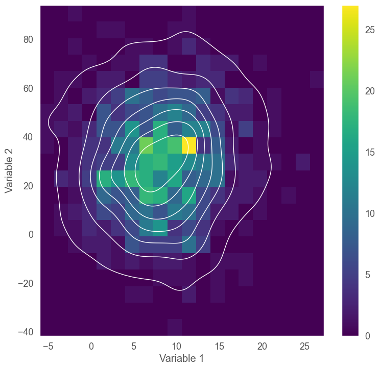
- Sometimes you have multiple variables that you want to visualize together as a distribution
- There are 2D analogs of both histograms and KDE plots
- One variable along each axis
- Counts or density still determine color
::::
::::col
::::
::::::
## Multivariate Distribution Creation
::::::{.cols style='align-items: flex-start'}
::::col
:::{.block name=Python}
- Histogram in Matplotlib
```python
plt.hist2d(xs, ys, bins=20)
```
- KDE plot easiest through Seaborn
```python
sbn.kdeplot(x=xs,
y=ys,
fill=True)
```
:::
::::
::::col
:::{.block name=R}
- Histogram through ggplot
```python
ggplot(data=df,
aes(x=xs, y=xs)
) +
geom_bin_2d()
```
- KDE plot through ggplot
```R
ggplot(data=df,
aes(x=xs, y=xs)
) +
geom_density_2d_filled()
```
:::
::::
::::::
# Understanding Brightness
## How Bright!
- Apparent brightness is the intensity of radiation (or reflected radiation) from a celestial body
- As measured by the observer, so generally from the Earth's surface
- Measured in units of watts per meter squared ($W/m^2$)
- For our Sun, this is about $ 1400\\ W/m^2$
- Clearly, the apparent brightness of other stars is going to be much, **much** less
- It is frequently useful to thus use a different scale, where instead we talk about _apparent magnitude_
## Apparent Magnitude
- System introduced around 150 BC!
- Hipparchus divided stars into six groups:
- Brightest were "1st magnitude"
- Faintest (that he could see) were "6th magnitude"
- These days we are much more precise, but have defined things to still largely adhere to these same ideas
- Measured on an inverted logarithmic scale
- Brighter objects have small magnitudes, and __they can be negative__
- A factor of 100 in brightness corresponds to a difference of 5 in magnitude
$$ m = -2.5\log\left(\frac{B_{obj}}{B_{Vega}}\right)$$
## Making Magnitudes Intuitive
- Smaller numbers mean brighter stars
- Numbers can be negative
- Smaller differences in magnitude correspond to larger differences in brightness
\begin{tikzpicture}%%width=100%
[xscale=.25, lbl/.style={rotate=90,right,font=\tiny\sf}]
\shade[rounded corners, left color=white, right color=black!50!blue] (-30,0) rectangle +(60,1);
\foreach \e in {-30,-20,...,30}{
\draw (\e,0) --+(0,-2mm) node[below, font=\sf] {\e};
}
\draw[Cyan,latex-] (-26.8,1) --+(0,3mm) node[lbl] {Sun(-26.8)};
\draw[Cyan,latex-] (-12.5,1) --+(0,3mm) node[lbl] {Full Moon(-12.5)};
\draw[Cyan,latex-] (-4.4,1) --+(0,3mm) node[lbl] {Brightest Venus(-4.4)};
\draw[Cyan,latex-] (-1.5,1) --+(0,3mm) node[lbl] {Sirius(-1.5)};
\draw[Cyan,latex-] (0.0,1) --+(0,3mm) node[lbl] {Vega(0.0)};
\draw[Cyan,latex-] (2.5,1) --+(0,3mm) node[lbl] {Polaris(2.5)};
\draw[Cyan,latex-] (6,1) --+(0,3mm) node[lbl] {Naked Eye Limit(6)};
\draw[Cyan,latex-] (10,1) --+(0,3mm) node[lbl] {Binocular Limit(10)};
\draw[Cyan,latex-] (26,1) --+(0,3mm) node[lbl] {4-meter telescope Limit(26)};
\draw[Cyan,latex-] (30,1) --+(0,3mm) node[lbl] {10-meter Telescope Limit(30)};
\end{tikzpicture}
## Activity! (10min)
:::incremental
- The file [here](../demos/bright_stars_10k.csv) catalogs most of the stars with magnitude brighter than 6.5 in our night sky (about 10 thousand)
- Visualize the distribution of right ascension vs visual magnitude with a standard scatter plot, a histogram, and a KDE plot. Can you see a two-lobed distribution?
- This distribution is actually caused by looking along the disk of the Milky way. The center of the Milky was is at a RA of about 18hr.
:::
# Asteroid Time
## Asteroids
::::::cols
::::col
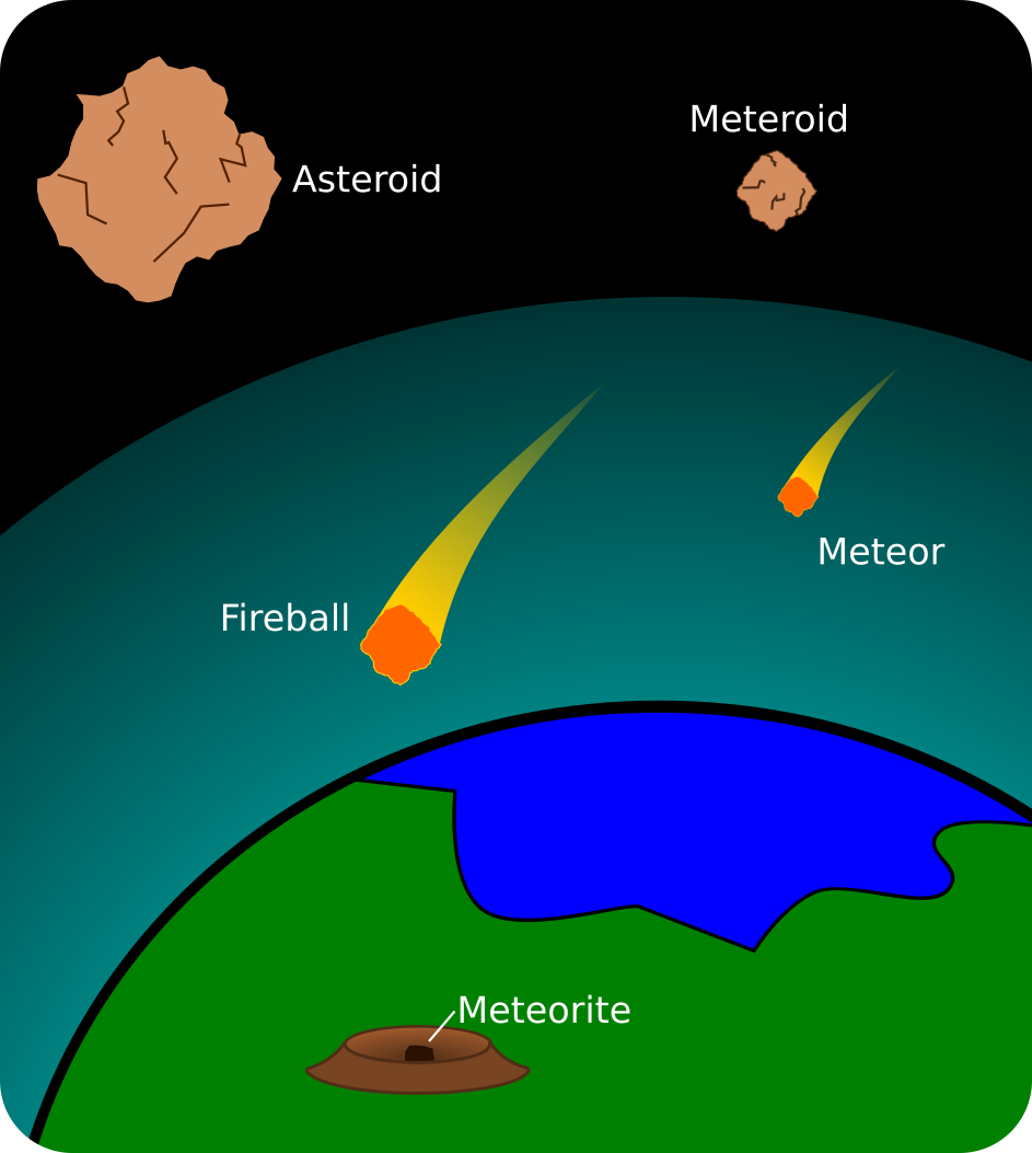
What are asteroids?
- Small (relatively) chunks of rock
- Maybe around a million are approximately 1 km across
- Many millions more are smaller
- Irregularly shaped
- Tiny = hard to see!
- "Primitive"
::::
::::col
{width=80%}
::::
::::::
## {data-background-iframe="https://www.asterank.com/3d/"}
## {data-background-iframe="https://eleanorlutz.com/mapping-18000-asteroids"}
## Why a Belt?
:::incremental
- Enough rocky material to form a body only about 3% the size of the Moon
- Gravity never brought it all together, like it did for the other inner planets. Why?
- **Jupiter**
- Played the role of a big bully
- Gravity broke apart any starting planetoids before they could really get going
- Still affects narrow bands of the belt today through _orbital resonance_
:::
## Orbital Resonance
- When the orbits of multiple objects sync up with one being a multiple of the other, they are said to be in _resonance_
- Resonance greatly boosts the interaction between the two bodies, with the most obvious effects on the smaller body
- Imagine pushing a child on a swing:
- Pushing in rhythm with the natural swing motion works best
- Could also push every other swing, or every 3rd swing, etc
- Pushing every 1/3 swing, for instance, would be highly counterproductive
## Unstable Resonance
::::::{.cols style="align-items: center"}
::::col
- Most often, resonances make orbits _unstable_
- The slow accumulation of boosts gives the smaller body more and more energy
- Generally results in the smaller body being ejected from the orbit
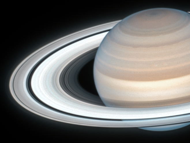
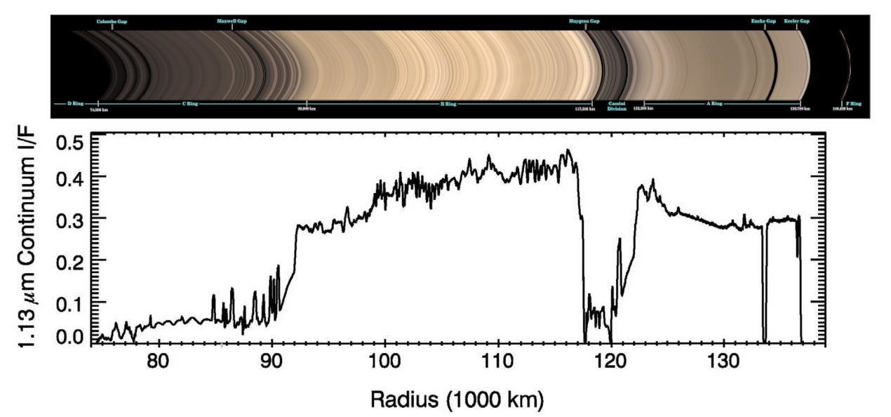
- This is the case with the Kirkwood gaps in the asteroid belt, and the Cassini division in the rings of Saturn
::::
::::col
{width=100%}
::::
::::::
## Resonance Pictured
- Mimas distance from Jupiter: 186,000 km
{width=100%}
## Stable Resonance
::::::{.cols style='align-items: center'}
::::col
- Resonance isn't always unstable though!
- Two body resonances can be stable if the ratios / orbits are such that they prevent the objects from getting too close
- Multiple orbits can influence each other to lock into a 4:2:1 resonance
- The most common is in the first three Galilean moons of Jupiter
::::
::::col
::::
::::::
## How long before we all die horribly?
## Ensuring Life
:::incremental
- Stated goal was to find 90% of asteroids 1 km or larger with near-Earth orbits
- **How do we know when that goal is reached?**
- Crater comparisons
- Rediscovery analysis
- Theoretical models
:::
## Latest Estimates
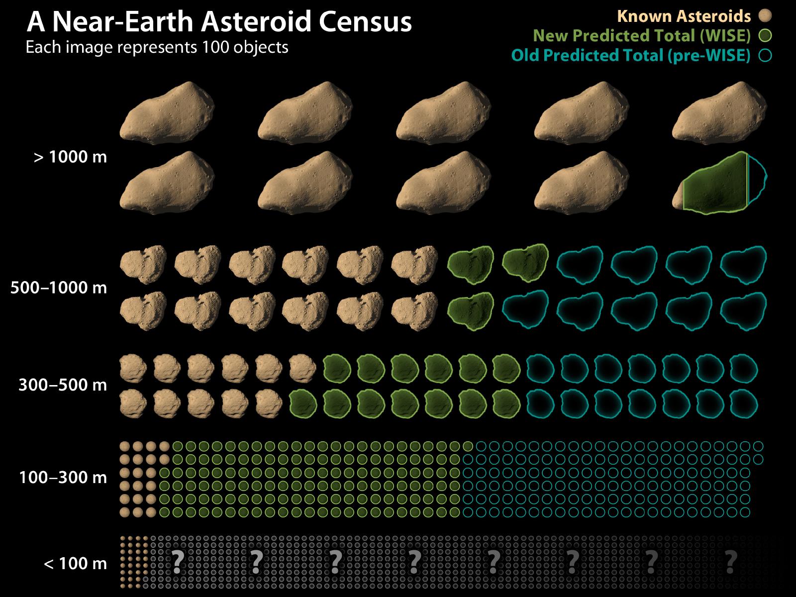{width=60%}
## Dissertation work
{width=70%}