---
title: "The Spooky Spectral"
author: Jed Rembold
date: January 30, 2025
slideNumber: true
theme: tokyo-night-light
highlightjs-theme: tokyo-night-light
width: 1920
height: 1080
transition: slide
p5js: true
---
## Announcements
- Homework 1 due on tomorrow night!
- Make sure you have at least attempted to export to a standalone HTML before the end of today!
- Example header yaml on next slide
- Please name the HTML after the problem number, e.g. `Prob1.html`
- All the groups look good and have all members joined, so just remember to upload!
- Debriefing form this weekend! Same link as the check-ins.
- Starting Unit 2: Stars today!
- Aiming to have HW2 and associated partners posted by the end of the weekend
- You'll have some time at the end of next Tuesday's class to meet up with your new partner
## YAML Template
- Essays can be made more attractive with some good choices in the YAML block at the top of your markdown/notebook
```yaml
---
title: Your essay title
author:
- Author_1
- Author_2
date: today
format:
html:
embed-resources: true
theme: cosmo
title-block-banner: true
---
```
- Many themes are possible. Full list [here](https://quarto.org/docs/output-formats/html-themes.html)!
## Today's Plan
- What is light?
- The electromagnetic spectrum
- Black Bodies and Planck's Law
- Wien's Law
- Fitting
# What is Light?
## How do we see?
- We see an object when light from that object reaches our eyes
- Either because the object itself emits light
- Or because that object reflected light

## Some Light Processing
- We get two pieces of information:
- The direction the light enters the eyes gives us positional information
- The color of the light gives us information about the composition of the light

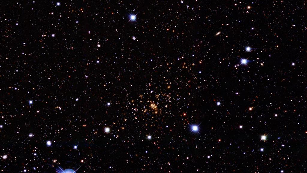
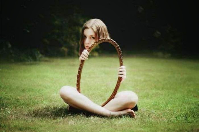
## Tricks of Light
- A single image gives no distance information
- Light can bend, which can confuse your brain
::::::cols
::::col
{.fragment .only-fragment data-fragment-index=0 width=100%}
{.fragment .only-fragment data-fragment-index=1 width=100%}
::::
::::col
{.fragment .only-fragment data-fragment-index=0 width=100%}
{.fragment .only-fragment data-fragment-index=1 width=100%}
::::
::::::
# The Electromagnetic Spectrum
## But what IS it?
- Light is, first and foremost, a wave
- Similar to an ocean wave, in that it travels in a direction
- Affects both electric charges and magnets "floating" atop itself
- Accordingly referred to as an _electromagnetic wave_
## Properties of Waves
\begin{tikzpicture}%%width=90%
%\draw[help lines] (0,-1) grid (10,1);
\draw[scale=0.5,domain=0:6*pi, samples=100, smooth, variable=\x, ultra thick, Cyan] plot (\x,{2*sin(\x r)});
\draw[|-|, very thick, Purple] (3/4*pi,-1.2) -- node[below] {Wavelength = $\lambda$} +(pi,0);
\draw[very thick, Purple, -latex] (8.2,.2) -- node[above] {Moving} +(2,0);
\draw[|-|, very thick, Purple] (-.2,0) -- node[above,sloped] {Amplitude} +(0,1);
\end{tikzpicture}
- All light waves move at the speed of light, $c$:
$$ c = 3\times 10^8 \text{ m/s}$$
- Amplitude corresponds to brightness
- Wavelength corresponds to color or portion of spectrum
## The Rainbow
\begin{tikzpicture}%%width=100%
\foreach \f/\c/\l in {7/black!50!violet/400,6/blue!50!violet!/440,5/blue/480,4/green/550,3/yellow/600,2/orange/630,1/red/720}{
\draw[\c,scale=0.5,domain=0:8*pi, samples=200, smooth, variable=\x, ultra thick] plot (\x,{sin(\f*\x r)-(2*\f)});
\node[\c] at (14,-\f) {$\lambda$ = \l \si{\nano\meter}};
}
\end{tikzpicture}
## You're (Mostly) Blind!
\begin{tikzpicture}%%width=100%
\pgfdeclarehorizontalshading{rainbow}{100bp}{
color(0bp)=(violet);
color(30bp)=(black!30!violet);
color(38bp)=(blue);
color(42bp)=(black!20!cyan);
color(46bp)=(green);
color(52bp)=(yellow);
color(58bp)=(orange);
color(65bp)=(red);
color(73bp)=(black!60!red);
color(100bp)=(black!50!red)
}
%Drawing the Bottom
\shade[shading=rainbow] (0,0) rectangle (9,1);
\draw[very thin] (0,0) rectangle (9,1);
\draw (0,0) -- (9,0);
\foreach \x in {0,0.5,...,9} \draw[thin] (\x,0) -- (\x,-0.1);
\foreach \x/\num in {0.5/400,3/500,5.5/600,8/700}{
\draw[semithick] (\x,0) -- (\x,-0.2)
node[below,font=\tiny] {$\SI{\num}{\nano\meter}$};
}
%Drawing the Top
\fill[black] (-1.5,3) -- (8.5,3) -- (9,3.5) -- (8.5,4) -- (-1.5,4) -- (-2,3.5) -- cycle;
\shade[shading=rainbow] (2.1,3) coordinate (x1) rectangle +(.35,1) coordinate (p2);
\foreach[count=\c] \x in {-1,0.8,...,8.1} \draw (\x,3) -- (\x,2.9) coordinate (\c);
\begin{scope}[font=\tiny, below]
\node at (1) {$\SI{1}{\pico\meter}$};
\node at (2) {$\SI{1}{\nano\meter}$};
%\node at (3) {$\SI{1}{\micro\meter}$};
\node at (4) {$\SI{1}{\milli\meter}$};
\node at (5) {$\SI{1}{\meter}$};
\node at (6) {$\SI{1}{\kilo\meter}$};
\end{scope}
\begin{scope}[right,font=\tiny,right,color=white, text width=1cm]
\node at (-1.0,3.5) {Gamma Rays};
\node at (0.4, 3.5) {X Rays\phantom{gamma}};
\node at (1.4, 3.5) {UV \phantom{gamma}};
\node at (3.0, 3.5) {\centering Infrared (IR)};
\node at (4.6, 3.5) {Microwaves \phantom{gamma}};
\node at (6.6, 3.5) {Radio \phantom{gamma}};
\node at (7.8, 3.5) {Long Radio\phantom{gamma}};
\end{scope}
%Connecting Bits
\draw[thin] (x1) ..controls +(-90:1.5) and +(20:1).. (0,1) coordinate(z1);
\draw[thin] ($(p2)-(0,1)$) coordinate (x2) ..controls +(-90:2.0) and +(170:1.2).. (9,1) coordinate(z2);
%Shading the Connecting Bits
\shade[shading=rainbow,opacity=0.2] (x1)..controls +(-90:1.5) and +(20:1).. (0,1) -- (9,1) ..controls +(170:1.2) and +(-90:2.0)..(x2)--cycle;
\end{tikzpicture}
## Everything the light touches...
- The general term _electromagnetic radiation_ describes all the wavelengths of electromagnetic waves, not just the visible ones we generally refer to as "light"
- Everything that emits or reflects radiation we can observe
- The visible bits are just a tiny fraction of the huge spectrum of possibilities
- Gives rise to different forms of astronomy:
- Optical
- Radio
- Microwave
- High Energy (Gamma/X Ray)
# Black Bodies
## Recipe: How to make some light
- How does one produce electromagnetic radiation?
- Microscopically: by accelerating electric charges
- Macroscopically: by making something hot
- By "hot" we just really mean "not 100% cold"...
- Heat excites the particles, bouncing them around and thus accelerating charges
- What wavelengths are emitted depends on the object's temperature
- Hot objects produce more radiation, so greater amplitudes overall
- Hot objects produce more radiation at shorter wavelengths
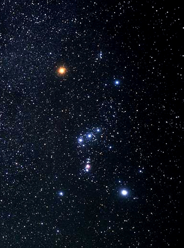
## A Shining Example
::::::cols
::::col
- The color of a star depends on its temperature!
- Brightness also depends on the temperature, but is also dependent on the star's size and distance from us
::::
::::col
{width=70%}
::::
::::::
## Planck's Law
- The brightness at a given wavelength emitted from a body in thermal equilibrium at some temperature is governed by _Planck's Law_:
$$ B(\lambda, T) = \frac{2hc^2}{\lambda^5} \frac{1}{\exp\left(\frac{hc}{\lambda k_B T}\right) - 1} $$
where
$$
\begin{aligned}
h &= 6.6261 \times 10^{-34} \text{ J}\cdot\text{s}\\
c &= 3\times10^8 \text{ m/s} \\
k_B &= 1.381 \times 10^{-23} \text{ J/K}\\
\lambda &= \text{wavelength in meters} \\
T &= \text{temperature in kelvin}
\end{aligned}
$$
## Planck's Law Visualized
\begin{tikzpicture}%%width=100%
\pgfmathdeclarefunction{planck}{1}{\pgfmathparse{1.19E-16/x^5*1/(exp(0.144/(x*#1))-1)}}
\begin{axis}[
domain=0:2E-5,
width=\textwidth,
height=6cm,
samples=50,
smooth,
xmin=0,
scaled ticks=false,
xlabel=Wavelength (m),
xticklabel style = {rotate=90},
ylabel=Intensity ($W/m^3\cdot sr$),
]
\addplot+[mark=none,ultra thick, Cyan] {planck(12000)};
\addlegendentry{12000 K}
\addplot+[mark=none,ultra thick, Yellow] {planck(10000)};
\addlegendentry{10000 K}
\addplot+[mark=none,ultra thick, Red] {planck(8000)};
\addlegendentry{8000 K}
\end{axis}
\end{tikzpicture}
## Nothing is Perfect
::::::cols
::::col
- Most things are not perfectly in thermal equilibrium, which will reduce the amount of radiation
- How well an object radiates is called its _emissivity_ ($\varepsilon$)
- Reduces the amount of radiation, but doesn't change wavelengths
- **Does** mean that often you'll have an extra unknown parameter though
$$ B(\lambda, T) = \varepsilon \cdot \frac{2hc^2}{\lambda^5} \frac{1}{\exp\left(\frac{hc}{\lambda k_B T}\right) - 1} $$
::::
::::col
\begin{tikzpicture}%%width=100%
\pgfmathdeclarefunction{planck}{1}{\pgfmathparse{1.19E-16/x^5*1/(exp(0.144/(x*#1))-1)}}
\begin{axis}[
domain=0:6000E-9,
scaled ticks=false,
samples=50,
smooth,
xmin=0,
ymin=0,
ticks=none,
xlabel near ticks,
ylabel near ticks,
xlabel=Wavelength,
ylabel=Energy Output,
axis lines=left,
axis line style={-latex},
height=7cm,
width=7cm,
]
\addplot+[mark=none, Cyan, ultra thick] {planck(12000)} node[pos=.6,right] {$\varepsilon=1$};
\addplot+[mark=none, dashed, Red, ultra thick] {.8*planck(12000)} node[pos=.7,left] {$\varepsilon=.8$};
\end{axis}
\end{tikzpicture}
::::
::::::
## Wien's Law
- Wien's Law relates the wavelength at the peak of the spectral black body curve to a temperature
- Can be useful if you only care about the temperature, and can observe the peak of the curve
- Has a very simple expression:
$$ \lambda_{peak} = \frac{2.8977\times10^{-3}\text{ m}\cdot\text{K}}{T} $$
in standard units, where $T$ is measured in kelvin
# Nonlinear Fitting
## Fitting Planck
- A spectra is an observable quantity
- Even if the star is far away so that it's brightness is lower, that just scales down the entire curve
- Spectra can thus be used to determine the approximate temperature of stars though either:
- Use of Wien's Law
- Fitting Plancks law directly
- Use of Wien's Law is usually simpler, but there can be times when you need to fit the entire blackbody curve
- Requires a nonlinear fit, but can still be done using common least squares algorithms (at least for the precision we need here)
## Least Squares Nonlinear Fitting (Python)
- In Python, you want `curve_fit` from `scipy.optimize` for this probably ([docs here](https://docs.scipy.org/doc/scipy/reference/generated/scipy.optimize.curve_fit.html))
- Need to define the function you want to fit, where the first parameter is the independent variable, and subsequent parameters are any desired fit parameters
- For Planck's law, that means wavelength is the first parameter, and amplitude and temperature the second
- When using `curve_fit` need to provide:
- The function name you want to fit
- The xdata
- The ydata
- An initial guess for any fit parameters (else starts at 1)
## Least Squares Nonlinear Fitting (R)
- In R, you'll likely want to use the `nls` function
- Give it a formula, using the column names where appropriate:
```R
brightness ~ A / wavelength^5 ...
```
- Specify what dataframe you are pulling the column names from:
```R
data=df
```
- Need to provide a list of starting values for the parameters
```R
start = list(e=100, T=1000)
```
## Fitting Demos
- For a demonstration, we are going to use the data [here](../demos/bbspec.csv)
- Noisy black body data with some general reduction in brightness
- Want to fit both the temperature and the emissivity
- We can compare our fits to what we'd have gotten from Wein's law