Absorption and Doppler

Jed Rembold

February 4, 2026

Announcements

  • I’m aiming to have HW2 feedback to you by the end of the week.
  • Homework 3 is due Monday!
    • Should have everything you need after today
  • We’ll start looking at HR diagrams on Monday

Recap:

  • We get two pieces of information when light enters our eyes: location and spectrum
  • Light is an oscillating EM wave, with many possible wavelengths
    • Visible from 400nm to 720nm
  • EM radiation comes from charges changing direction and speed
    • Hotter objects:
      • Produce more radiation
      • Produce “bluer” radiation
    • Planck’s Law models this relation: \[ B(\lambda, T) = \frac{2hc^2}{\lambda^5}\frac{1}{\exp\left(\frac{hc}{\lambda k_B T}\right) - 1} \]

Today’s Plan

  • Atomic spectral lines
    • Emission
    • Broadening
    • Absorption
  • Doppler

Spectra and Composition

  • Objects with thermal spectra are generally dense (wood, rocks, people, metals, stars, etc.)
  • A perfect “blackbody” spectrum would only give us information about the temperature
  • Diffuse gases though can have more complex spectra, such that we can actually get information about chemical composition
    • Interestingly, this information also can help us identify some aspects about motion
    • Why is gas special?

Emission

Life of an Electron

  • Electrons orbit around the nucleus of an atom
  • Only allowed in certain areas, which correspond to different energy levels
  • The height of each energy level is determined by the atomic properties of the nucleus

Energy

Fingerprinting Light

  • The discrete energy levels result in line spectra
  • These spectra are unique for each atom and molecule, so they work as fingerprints!

Broadening

Seems Sus

  • Stars (especially the surface) are made almost entirely of hydrogen
  • So why do we get a (mostly) blackbody curve when looking at stars, and not sharp hydrogen emission peaks?

Stars \(\neq\) Gas Lamps

  • Atoms in close proximity to one another influence each other’s energy levels

Evolution of Spectra

Absorption

Absorption Spectra and Goldilocks

  • What if we have a cooler, diffuse gas, but with blackbody radiation shining on it?
  • Some of the radiation will be absorbed
  • Only the “just right” wavelengths corresponding to certain energy steps

Sample Case: Hydrogen

That Spectra is Stellar!

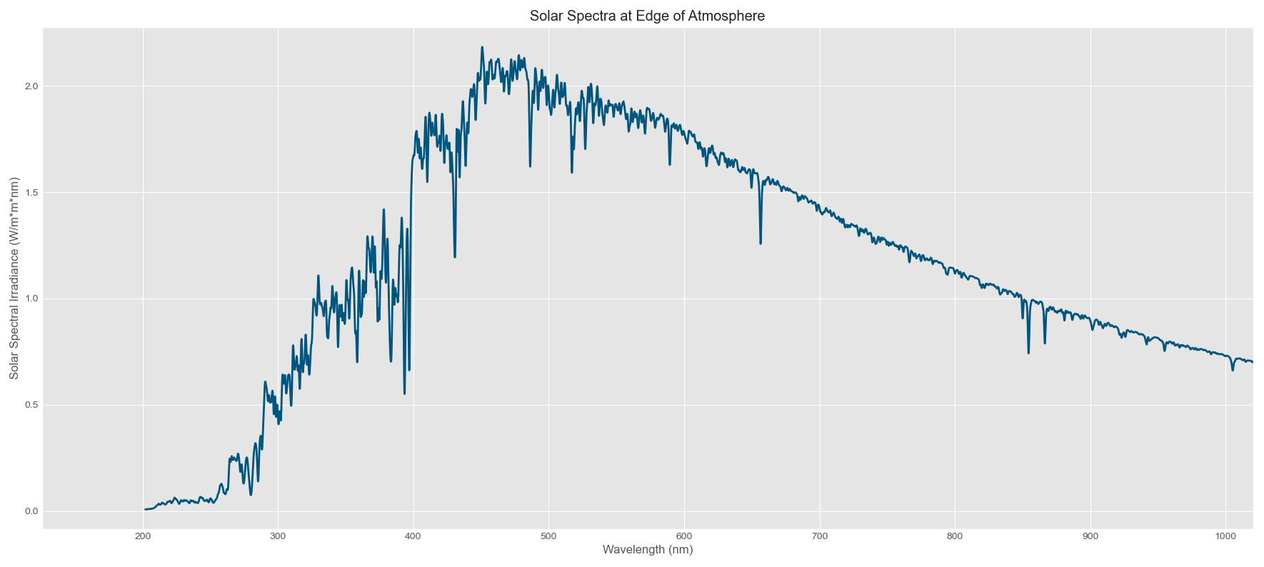
  • Hot gases in the surface regions of a star emit a blackbody spectrum, depending on their temperature
  • Slightly cooler gases further out absorb some wavelengths, giving rise to absorption lines

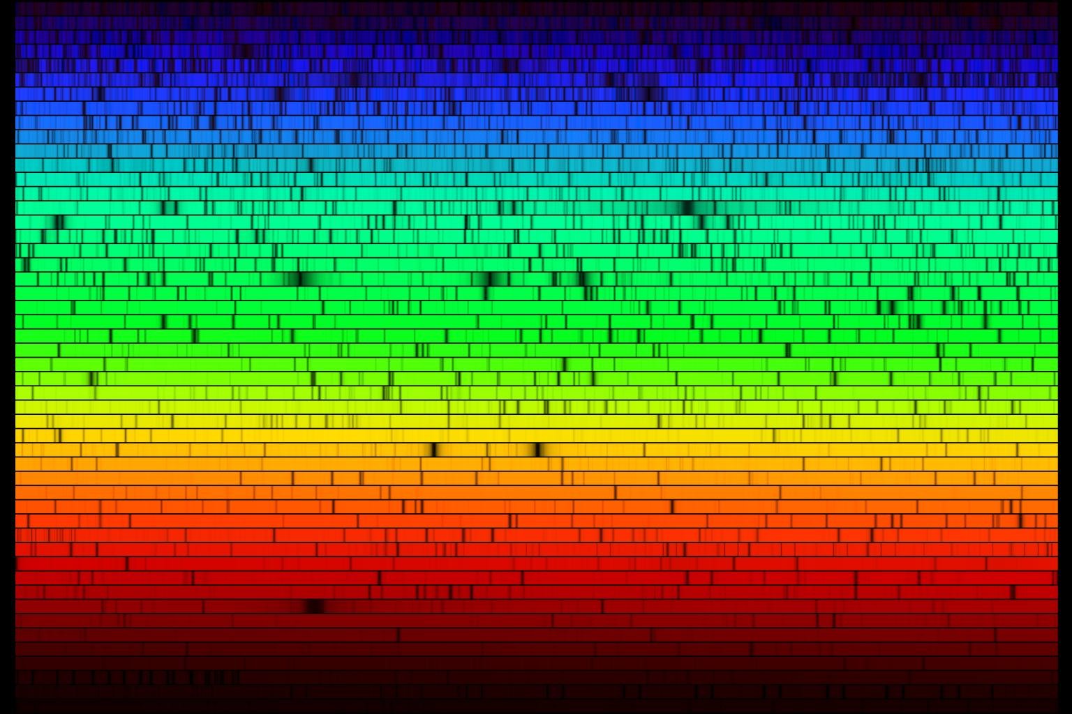
Viewing Absorption Differently

But wait, there’s more!

Doppler

The Doppler Effect

  • The Doppler effect affects all types of waves, including light!
  • Approach waves get compressed (smaller wavelengths)
  • Receding waves get stretched (larger wavelengths)

Putting Numbers to It

For our purposes: \[ \frac{\lambda_{obs} - \lambda_{rest}}{\lambda_{rest}} = \frac{V}{c} \] where:

  • \(\lambda_{obs}\) is the wavelength you, the observer, see
  • \(\lambda_{rest}\) is the normal wavelength you’d see if the object was not moving
  • \(V\) is the speed of the light source relative to you
    • Negative if coming towards you
    • Positive if moving away from you
  • \(c\) is the speed of light

Astronomy Implications

  • We can measure radial speeds of objects!
  • Approaching objects are blueshifted
  • Receding objects are redshifted

Finding and Measuring Absorption Peaks

Maximum Redshift

  • Stars are considered “hypervelocity stars” if they have radial speeds of around 500 km/s or higher
  • Take a moment to compute how much of a shift this would cause in the \(H_\alpha\) line usually at 656.464 nm.

\[\Delta\lambda = \frac{500\times10^3}{3\times10^8}\times 656.464 = 1.094\]

  • The shift would be only a single nanometer!
  • Finding the peaks isn’t difficult, as they are largely where we expect
  • Measuring the slight differences is far more tricky

Gaussians

  • Measure peak placement precisely involves fitting a model to the peak
  • One of the most common is that of a Gaussian: \[ g(x) = H + A\exp\left(\frac{-(x-x_0)^2}{2\sigma^2}\right) \] where
    • \(H\) is the offset or shift of the baseline
    • \(A\) is the peak height above the baseline (can be negative)
    • \(x_0\) is the \(x\) at which the peak is centered
    • \(\sigma\) is the spread of the peak

The Continuum

  • Peaks often show up on areas of the blackbody spectrum that are heavily sloped
  • Fitting them well requires “flattening”, or normalizing out this background continuum
  • Most common approach is to fit a line or polynomial to just the background (not the peak!) and then divide the entire background by this signal
  • If done well, you should get a clean peak sitting on a level surface, ready for fitting
  • For velocities or identifying chemical composition, determining \(x_0\) is the most important, as that is the wavelength the peak is centered at

Example Using Solar Spectra

  • To illustrate this approach, let’s investigate the \(H_\alpha\) line in the solar spectra given here
  • Want to:
    • Establish there is a peak approximately where we expect it
    • Normalize the background
    • Fit a gaussian to determine peak location

Velocity Computing

  • You can technically compute a velocity for each peak individually
  • The spectrum will generally have many peaks
  • Don’t just average them! Fit a line to them: \[\lambda_{obs} = \left(\frac{V}{c} + 1\right)\lambda_{rest} \]

λrest λobs

// reveal.js plugins // Added plugins ,