---
title: "Transit Techniques"
author: Jed Rembold
date: March 4, 2025
slideNumber: true
theme: tokyo-night-light
highlightjs-theme: tokyo-night-light
width: 1920
height: 1080
transition: slide
p5js: true
---
## Announcements
- Welcome back!
- I was slow getting the weekend checkins available, and then somehow put in the wrong dates at first. So I've given you until the end of _today_ to get a checkin submitted if you haven't yet
- HW3 deadline pushed until next Tuesday night, to account for slow feedback
- Quiz 1 will be handed back and discussed on Thursday. I still need to record scores.
## Recap
- The Lomb-Scargle Periodogram is an approach that works well for non-uniform data
- Requires you to specify the range of angular frequencies / frequencies / periods that you want to computer the power over
- Aliasing will generally be a factor you need to content with
- Planets and their parent star technically orbit their shared center of mass
- Causes the star to "wobble", which can be measured!
- Astrometric method looks for the shift in the star relative to background stars
## Discussing Today
- Doppler method for wobbles
- Planet properties from wobbling methods
- The Transit Method
- If time: extra numerical techniques
# Understanding Wobbles
## Wiggle Wiggle
- Often, we are not viewing the plane of an exoplanetary system directly from the top
- How we see this "wiggle" from Earth depends on how the planets orbit is oriented relative to us
- A perfectly "top down" view would have us seeing the planet making little circles
- A perfectly "side" view would have us seeing the planet move towards us and away from us on the left and right sides
- In general, it is easier for us to detect and measure the forwards and backwards motion, but instruments like Gaia _can_ detect the tinier circular motion for some systems
## Full Example
## Doppler Wiggle
- The idea is to monitor the dominant frequency of light emitted over a period of time
- Should result in a sinusoidal curve as the star wiggles toward and then away from us
- The amount of wiggle will depend on **both** the mass of the orbiting planet **and** our perspective
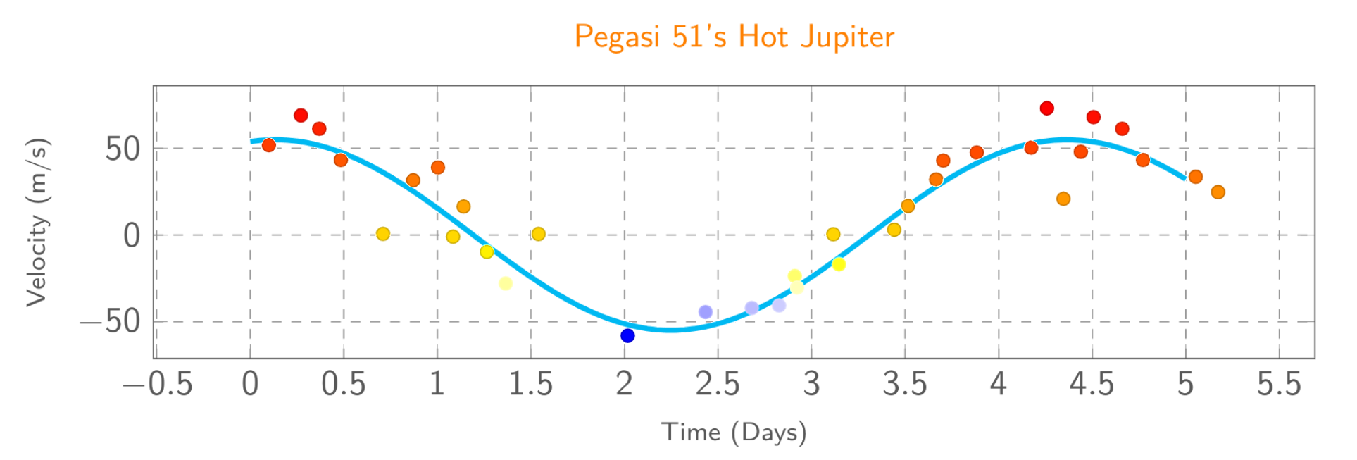{width=70%}
# Determining Planetary Mass
## Beginning to extract planetary properties
- In general, to understand any exoplanet, you must first understand its parent star
- This is often **considerably** easier, since the star is big and bright
- Several parameters in particular are useful to know:
- The mass of the star
- The size of the star
- Both generally require knowing the distance to the star, but otherwise can be worked out from luminosities or location on the HR diagram
## Planetary Period and Distance
- If you have the period of the star, then you have the period of the planet
- Both move in lockstep about the center of mass
- If you have multiple planets, you can separate the different components from the stars motion
- Extracting the distance to the planet / semimajor axis requires application of Kepler's 3rd law along with the center of mass location:
$$\text{Kepler's 3rd: } \frac{GM_{tot}}{4\pi^2} = \frac{a^3}{p^2} \qquad\qquad\text{Center of Mass: } M_1a_1 = M_2 a_2 $$
## Planetary Mass (Part I)
- Combining $a_1$ and $a_2$:
$$ a = a_1 + a_2 = a_1\left(1 + \frac{a_2}{a_1}\right) = a_1\left(1 + \frac{M_1}{M_2}\right) = \frac{a_1}{M_2}\left(M_2 + M_1\right) = \frac{a_1 M_{tot}}{M_2} $$
- Plugging into Kepler:
$$ \frac{GM_{tot}}{4\pi^2} = \frac{1}{p^2} \left(\frac{a_1 M_{tot}}{M_2}\right)^3 $$
- If you know $a_1$ by direct observation, then you are done, and can solve for $M_2$!
- Otherwise you need to write $a_1$ in terms of a velocity
- If you assume mostly circular orbits:
$$v_1 = \frac{2\pi a_1}{p} \quad\Rightarrow\quad a_1 = \frac{v_1 p}{2\pi}$$
## Planetary Mass (Part II)
- Plugging that back into Kepler:
$$ \frac{GM_{tot}}{4\pi^2} = \frac{1}{p^2} \left(\frac{a_1^3 M^3_{tot}}{M^3_2}\right) $$
. . .
$$ \frac{GM_{tot}}{4\pi^2} = \frac{1}{p^2} \frac{M^3_{tot}}{M^3_2} \left(\frac{v_1 p}{2\pi}\right)^3 $$
. . .
$$ \frac{GM_{tot}}{4\pi^2} = \frac{1}{p^2} \frac{M^3_{tot}}{M^3_2} \frac{v_1^3 p^3}{8\pi^3} $$
. . .
$$ G = \frac{M^2_{tot}}{M^3_2} \frac{v_1^3 p}{2\pi} $$
. . .
$$ M_2 = \left(\frac{M^2_{tot}}{G}\frac{v_1^3 p}{2\pi}\right)^{1/3} $$
## Some Caveats
- The true velocity is only what is measured at the peak of the Doppler curve if you are viewing the orbit **perfectly** edge-on
- In general:
$$ v_{obs} = v_1\sin(i) $$
where $i$ is the _orbital inclination_ ($0^\circ$ if viewing face-on, or $90^\circ$ if viewing edge-on)
- If the inclination angle in unknown, then technically you are finding a minimum mass
- If the eccentricity is known, then:
$$ M_2 = \left(\frac{M^2_{tot}}{G}\frac{v_1^3 p}{2\pi}(1- \epsilon^2)^{3/2}\right)^{1/3} $$
## Practice
- The file [here](../demos/planet_mass_activity.csv) contains velocity information determined from the redshift/blueshift of a star with a single planet orbiting it.
- You can assume the planet is traveling in a mostly circular orbit.
- You know that the parent star has a mass of $2\times10^{30}$ kg.
- Determine:
- The period of the planet
- The minimum mass of the planet
# Determining Size
## Full Example
## Transits
- If a planet system is oriented towards us **just right**, then on occasion we should see a planet pass in front of the star
- This is a much narrower restriction than what we had with Doppler, which was just that we needed the planet system to be tilted toward or away from us at all
- The effect is similar to a solar eclipse on Earth
- Light from the Sun/star is blocked for a certain amount of time
- Some important differences owing to perspective though:
- Our Moon is of a size and distance that it can totally block our Sun. That is not the case for exoplanets
- Our Moon orbits Earth, not the Sun as exoplanets do
- We **can** observe these same effects for Mercury and Venus though
## Venus Transit {data-background-iframe="https://www.youtube.com/embed/ku7YjMol1k4"}
## Transit Info
::::::cols
::::col
- The most important information from a transit involves the depth of the brightness reduction
- This directly correlates to the ratio of the cross-sectional area of the star and the planet
- Duration of transit can give other useful information, but tougher to extract
- Planet speed
- Inclination angle
::::
::::col
\begin{tikzpicture}%%width=100%
[scale=.7, every node/.style={font=\sf}]
\draw[-latex] (0,0) -- node[pos=.3,above,sloped,font=\sf\scriptsize] {\% of Light} (0,4);
\draw[-latex] (-.5,3) node[left] {100\%} --(5,3) node[above] {\scriptsize Time};
\draw[Cyan, ultra thick] (0,3) -- (1,3) -- (1.5,1) -- node[midway,below] {95\%} (2.5,1) -- (3,3) -- (4,3);
\end{tikzpicture}
::::
::::::
## Planetary Radii
::::::cols
::::col
- As long as your transit shows a flat portion at the bottom of the dip, then you know that the planet fully covered the star
- Then you can work out the planet radius
::::
::::col
$$\begin{aligned}
\text{% of light } &= \frac{\text{Area of planet}}{\text{Area of star}} \\
&= \frac{\pi R^2_p}{\pi R^2_s} \\
&= \left(\frac{R_p}{R_s}\right)^2
\end{aligned}$$
::::
::::::
# Dealing with Noise
## Averaging out Noise
- There will often times be noise that detracts from or obscurs a signal
- In astronomy, this commonly comes from thermal sensor noise or atmospheric effects
- Can show up in any signal though where measurement-to-measurement variations obscur a longer pattern in the signal
- One method to try to eliminate this noise is with Fourier Transforms
- Set all signals in the frequency domain to 0 except your main signal and then inverse it back to the time domain
- We can't do that (easily) for non-uniform measurements though
- What other options might we have?
## Rolling Averages
- A _rolling average_ computes an average for **each** point in a data series, usually taking into account a certain number of observations on either side of the point in question
- This is the same result as convolving a square wave with a certain width with the noisy signal
- The size of the square wave or "window" directly affects the amount of smoothing that will be seen: bigger windows smooth things more
- Algorithm can vary, but the basic algorithm is just looking a position of data within the series, so it does **not** account for data spacing.
- Data ordering matters!
- This may still be fine for some non-uniformly sampled data, provided the window in only marginally larger than the average spacing
## In Python: Direct Convolution
- Doing the convolution directly means constructing the square wave in Numpy and then using Numpy's convolution function
```python
window = np.ones(size) / size # necessary to scale!
out = np.convolve(signal, window)
```
- The output by default has length $L_{signal} + L_{window} -1$, so if you want to plot it against your original times, you need to mask off the last parts
- You **really** need to ensure your signal points are ordered by time for this to work! The easiest way to achieve this is with `np.argsort`:
```python
sorted_idxs = np.argsort(ts)
sorted_times = ts[sorted_idxs]
sorted_signal = signal[sorted_idxs]
```
## In Python: With Pandas
- Assuming you already have your data in a dataframe, you **still need to ensure it is ordered!**
```python
df = df.sort_values('ts')
```
where `ts` is whatever column you want to sort by
- This just reorders the index, so be aware if you try to extract just a column by itself
- Computing the rolling average is then straightforward:
```python
df['rolling'] = df.sig.rolling(wsize).mean()
```
where `sig` is whatever column you are computing the average over, and `wsize` is the size of the window you want
## In R: With Zoo
- You still want to ensure your data is ordered! Can use `arrange` if using Tidyverse
```R
df <- arrange(df, colname)
```
- Easiest to use `rollmean` from the `zoo` library for the rolling averages
```R
library(zoo)
df <- df %>%
mutate(
rolling = rollmean(colname, k=wsize, fill=NA)
)
```
## Rebinning
- Sometimes, you just need to take non-uniformly sampled data and cast it into something more consistent
- If the data is noisy, this can also help cut down on the noise
- The idea is to compute new, evenly spaced bins, and then compute the mean (or median) of all the points that fall within that bin
- Some bins might not contain any points, and that is ok! They can just get assigned null values.
- You could then proceed to do anything you would do with uniformly sampled data: Fourier transforms, further rolling averages, etc
## Rebinning in Pandas
- You can either specify the bins with a list, or have Pandas compute the bins for you given a desired number of bins
- I find the former better when I have specific data that I'm trying to rebin
- Key function in Pandas is `pd.cut`, which takes several arguments:
- The array that you are trying to bin by
- The bins or number of bins that you desire
- How you want to handle the bin labels
```python
bin_labels = pd.cut(df.ts, bins=np.arange(0,10,0.1),
labels=False)
```
- This gives labels as **indexes**. I prefer to know the start of the bin, so I multiply by the bin step size
## Rebinning in R
- Similar to Pandas, you can use the `cut` or `ntile` functions to compute a binning:
```R
df %>% mutate(
bins = cut(colname, breaks=seq(0,10,0.1)
)
```
gives your bins as intervals, whereas
```R
df %>% mutate(bins = ntile(colname, n=100))
```
gives the bins as integers