Full Example

Transits

• If a planet system is oriented towards us just right, then on occasion we should see a planet pass in front of the star
  • This is a much narrower restriction than what we had with Doppler, which was just that we needed the planet system to be tilted toward or away from us at all
• The effect is similar to a solar eclipse on Earth
  • Light from the Sun/star is blocked for a certain amount of time
• Some important differences owing to perspective though:
  • Our Moon is of a size and distance that it can totally block our Sun. That is not the case for exoplanets
  • Our Moon orbits Earth, not the Sun as exoplanets do
• We can observe these same effects for Mercury and Venus though

Venus Transit

Transit Info

Planetary Radii

Non-sinusoidal oscillations

• Recall that we originally motivated Fourier Transforms by maintaining that they could be used on any periodic motion
  • Because anything periodic could be written as a sum of sine waves
• But there is a price in practice
• We are going to see peaks from all of those major contributions
  • These are called harmonics

Fourier Series of a Square Wave

FFT of Transits

• Those extra peaks are not aliases, they are harmonics
• Technically needed to “center” the signal around 0 to get the above

Lomb-Scargle of Transits

Frequency Spread

• There is another problem here beyond just “I don’t want to deal with all of these peaks”
• Each component peak represents a bit of the signal
• By having many peaks, we are essentially smearing the signal out over many more peaks
• This lowers the power of all the peaks, making it harder to detect a peak in the first place

Phase Folding

• Periodograms are excellent for determining the frequency / period of hidden signals, but they don’t let you see those signals

• Alternatively, could guess a period and then use that to “fold” the signal back in on itself

  • Snippets of the signal that may have been captured by very different observations get properly aligned or stacked
  • Noise can get properly averaged out, improving signal to noise ratios

• The phase of the signal describes how far is signal is through its period

• Calculating phase is a classic example of using the modulo operator:

  phase = times % period
  normalize_phase = phase / period

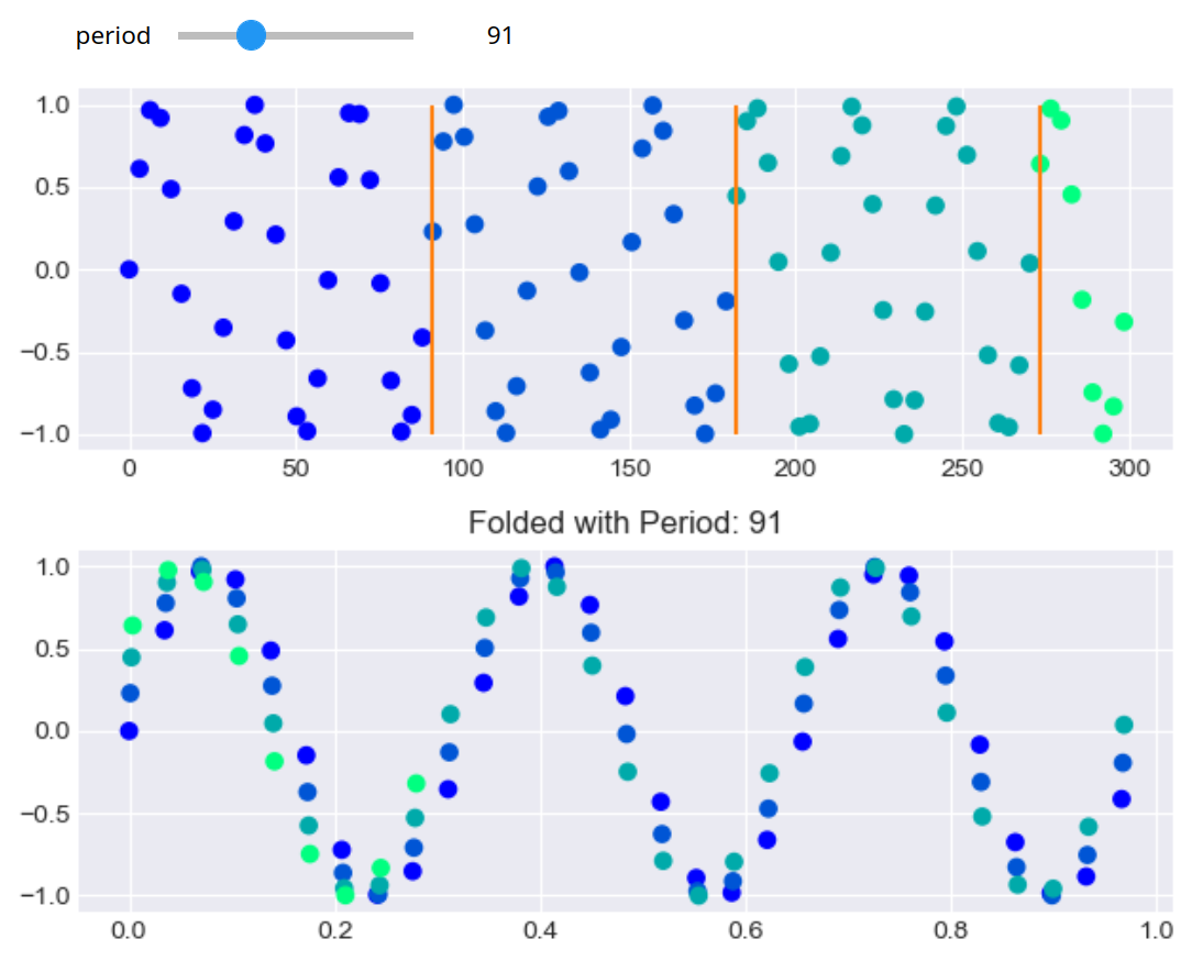
Visual Phase Folding

• Often times you’ll see the phase normalized by the period, so that it starts at 0 and ends at 1
• Be careful! Folding at integer multiples of the true period may look clean, but will contain more than a single oscillation
• Notebook Demonstration (requires the ipywidgets package)

Box Least Squares (BLS)

• In 2002, Kovàcs, Zucker, and Mazeh published the original BLS, or Box Least Squares, approach, and it has been further optimized is the years since
• BLS emphasizes a grid-search approach, sliding a rectangular box over a phase-folded signal
• The goal is to find where the biggest difference between the average inside the box and the average outside the box exists
• Grid-search = brute force method
  • Looks at a wide variety of periods (for the folding)
  • Transit durations (for the size of the box)
  • Start points (for how quickly to move the box)

Step 1: Removing Long-term Trends

• BLS is very sensitive to long-term star variability (slowly brightening or dimming)
• If the signal has a slight slope, the box will always “fit” better at one end
• Several approaches:
  • Fit a high-order polynomial
  • Do a rolling median average
    • Just need to make sure that the window is much larger than any possible transit
• Once flattened, subtract the mean to zero-center the data

Step 2: The Grid Search

• We have several parameters to vary in our grid search
• What periods to test (phase-fold)
  • Really, we want to do this in frequency space for nice linear steps
  • A good rule of thumb is to take steps no larger than \[ \Delta f = \frac{0.01}{t_{span}} \]
  • Ranging from periods of about 0.5 days to 20 days
• What durations to test (size of box)
  • This is a fraction of the period, usually between 0.01 to 0.1 or 0.15

Step 3: Phase-Folding and Binning

• For every frequency/period in the grid, we compute a normalized phase for the data and reorder it
• To greatly speed up the next step, we rebin the phase space data, usually into 200 - 1000 bins
• For each bin, need to track:
  • The weight: count of number of points that went into that bin
  • The average signal of all points in that bin

Step 4: The Scan

• For the specific period, a box of width L (the duration) is slid through the bins
• At each position, the Signal Residue is computed
  • \(s\) = sum of the signal in the box
  • \(r\) = sum of the weights in the box
  • \(N\) = the total weight overall (number of points)
  • \(S\) = the power \[ S^2 = \frac{s^2}{r(N-r)} \]
• Keep the highest \(S\) (but write down the \(L\) and position as well)

Step 5: Periodogram Construction

• Can then construct the periodogram as usual
  • Frequency/Period across the bottom
  • \(S\) on the y-axis