See Me Rolling

Jed Rembold

March 4, 2026

Announcements

Homework 7 is out and due on Monday!
Everything you’ll need you have after today
I am continuing my quest to get caught up on grading
- Adding this new content this week slowed it down, but I think the new content is worth it

A transit happens when a planet passed between its parent start and our line-of-sight
The dip in brightness gives us information about the size of the planet \[\text{Fraction of light lost} = \frac{R_{planet}^2}{R_{star}^2}\]
The shape of transits means that we see many harmonics when using FFT or Lomb-Scargle methods, which come from the Fourier series components
A better method with transits is to use a Box Least Squares method

BLS in sensitive to changes in the star brightness that are not due to a transit
So we need to level everything else out, without affecting the transit drop
Could fit a high-order polynomial, but those are usually very impacted by possibly outliers
A better, and arguably simpler approach, is to subtract a rolling median

A “rolling” statistic looks at a surrounding window for each point in a data set, and computes some descriptive statistic over that window
- Rolling means/averages or rolling medians are probably the most common
Main choice is in the size and placement of the window
- Bigger windows have bigger effects on the resulting data (more smoothing)
- Windows can be centered on a point, come before, or come after
Algorithms can vary, but the basic algorithm is just looking at position of data within the series, so it does not account for data spacing.
- Data ordering matters!

You should always ensure your data is sorted before computing a rolling statistic on it
In Python, with pandas:
```
df = df.sort_values(colname)
```
In R, with Tidyverse:
```
df <- arrange(df, colname)
```

Easiest to use rollmean (or rollmedian) from the zoo library

library(zoo)

df <- df %>% 
  mutate(
    rolling = rollmean(colname, k=wsize)
    )

When you compute a rolling statistic, points near the edge of the dataset will not have a full window, leading no NaNs or NAs
The BLS algorithm does NOT handle these well
In Python, can set min_periods=1 to have the window “grow” out on edges
In R, can set fill='extend' to have it pad out NA with the closest value
Either is fine so long as your transit isn’t super near the edge of your data

With transits your goal is to choose a window that is definitely bigger than a possible transit duration (which is usually less than a couple hours)
If your window gets too big, it will start doing a bad job flattening the data (wiggles or slopes will remain)
To flatten, you want to subtract the rolling median from the original data
This will mostly zero it out as well, but it is then never a bad idea to subtract the entire median from the data to ensure it is fully “zeroed”

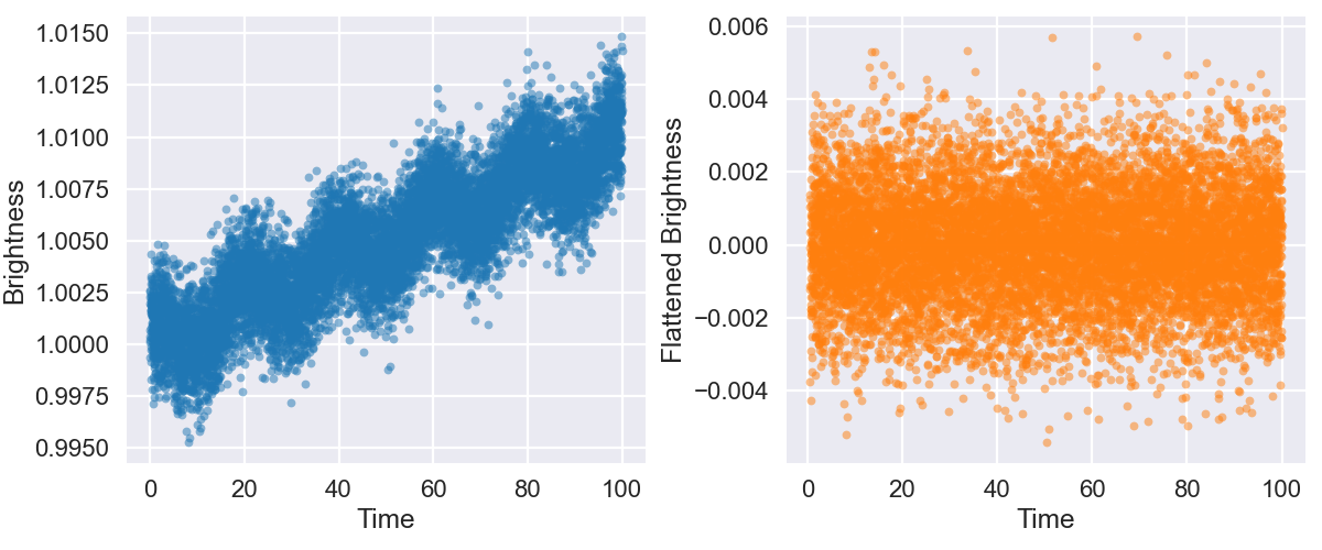
The file here depicts a brightness curve over 100 days
There is evidence both of a general slope to the data and some oscillations unrelated to anything of interest
Flatten the signal out and zero-center it, as if you were preparing it for BLS

We have several parameters to vary in our grid search
What periods to test
- Really, we want to do this in frequency space for nice linear steps
- A good rule of thumb is to take steps no larger than \[ \Delta f = \frac{0.01}{t_{span}} \]
- Ranging from periods of about 0.5 days to 20 days
What durations to test (size of box)
- This is a fraction of the normalized phase, usually between 0.01 to 0.1 or 0.15
The number of bins we want to break the phase space up into
- Generally numbers of bins between 200 and 1000 work well

The output of bls_search includes both period and power columns, so creating a periodogram is easy
You are still likely to see multiple peaks here
- Recall how with phase folding things still seemed to line up “somewhat” when we were at integer multiples of the true period?
Same advice applies at looking for the largest peak that is near the lowest frequencies
Can determine with a peak_finder or, if the largest, just filter it out of the table

Recall that the BLS algorithm computes \(s\) and \(r\) values as it slides along each phase-folded signal. These actually have all the depth information hidden within them
For a given peak period, you can compute the depth of the signal with: \[ \text{Depth} = \frac{|s|}{r} + \frac{|s|}{N-r} \] where \(N\) was the total weight (number of observations)
You can and should probably check this against a smoothed, phase-folded version of the signal

BLS also scores the best fitting duration and location
Both are given in terms of the bins, so need to take into account the number of total bins that you used \[ \text{Duration} = \frac{\text{duration in bins}}{N_{bins}} \cdot \text{Period} \] \[ \text{Starting Phase} = \frac{\text{start bin}}{N_{bins}} \]
These can also be compared/checked against a smoothed, phase-folded version of the signal