Logistic Regression
Jed Rembold
March 11, 2026
Announcements
- HW8 is out!
- If you had issues getting HW7 submitted, make sure it is submitted ASAP
- If you want to take into account feedback to make small updates to HW4-7, that is fine, but make sure HW4 is updated by the end of today
- Partner Debriefing for Unit 3 is up until the end of Friday, don’t forget!
Recap
- Determining the shape of an object while inside it is a non-trivial task
- Distance measurements are vital to piece together the shape of the Milky Way
- Parallax measurements cover a very tiny portion of the
Milky Way, and thus other methods are necessary
- Main sequence fitting
- Cepheid variables have their brightness fluctuate in a way that is related to their luminosity
- Galaxies largely form as the result of large regions of mostly hydrogen gas collapsing inwards under gravity
- Galaxies come in three main “flavors”:
- Spiral Galaxies
- Elliptical Galaxies
- Irregular
Discussing Today
- Evaluating classification models
- Basic data prep in Python and R
- Our first model: Logistic Regression
- Building, training, and testing models in Python
- Building, training, and testing models in R
Judging Classifications
Fitting vs Classification
- We’ve seen several ways to fit models to data already
- Basic linear fitting
- Non-linear model fitting
- Both give a prediction of a continuous variable given some inputs
- Classification is about predicting a discrete variable (or factor)
Techniques over Theory
- In this class, I’m going to focus on techniques over the underlying mathematical theory
- Problem-solving is often a game of abstraction, and using techniques
as tools can help with that
- You don’t need to know the details of how a least-squares fit is done to make use of it
- For rigorous work, you should be aware of at least the basic theory underlying a technique, at least well enough to know if you are misusing it
- I am going to present the machine learning techniques in this unit
in a similar, technique over theory fashion
- We have other classes if you want a deep dive into this sort of content!
Be Positive!
- With regression fitting, we commonly have an idea of a residual, which measures how far from an actual value our prediction came
- A similar idea won’t hold for classification, because we either correctly classified the point, or we didn’t
- Instead, for a binary classification (A or B), predictions would
fall into 1 of 4 different bins:
- True positive: An observation that should have been in category A, which our model predicted was in category A
- False positive: An observation that should have been in category B, but which our model predicted would be in category A
- True negative: An observation that should have been in category B, which our model predicted was in category B
- False negative: An observation that should have been in category A, but which our model predicted would be in category B
Confusion Matrix
- For either binary classification or multinomial classification, a confusion matrix is often the best method to summarize model prediction results visually
- Compares actual categories across one axis to predicted categories across the other
- Each bin contains a count of how many observations with that actual value were predicted
Making Comparisons
- Comparing just confusion matrices can be ambiguous
- Which model best classified the data of the below options?
Precision and Recall
- For a binary classification, there are clear methods of evaluating a model
- Precision is a measure of how much you can trust the model if it claims a positive \[ \text{Precision } = \frac{TP}{TP + FP} \]
- Recall is a measure of how reliably the model finds all the positive observations \[ \text{Recall } = \frac{TP}{TP + FN} \]
Accuracy
- One of the simplest extensions of this to multinomial data is to use accuracy
- Accuracy is a probability that, for a random observation, the predicted class is correct \[ \text{Accuracy } = \frac{\text{Diagonal counts}}{\text{Total observations}} \]
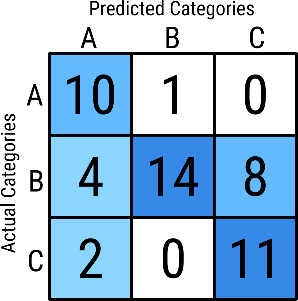
\[\begin{aligned} \text{Accuracy } &= \frac{10 + 14 + 11}{11 + 26 + 13} \\ &= \frac{35}{50} \\ &= 0.7 \end{aligned} \]
Accuracy Issues
- If your data has far more of one category than others, accuracy might hide issues
- Suppose your model predicts the dominant category really well, but other categories terribly
- The odds of selecting an observation from the dominant category are
high, and thus the accuracy will also look high
- But you may be doing a terrible job of classifying the minority classes!
- We’ll introduce some alternatives going forward, but let’s work with accuracy for the time being, despite its flaws.
Supervised Machine Learning
- There are a host of ways classification problems can be solved, but many modern approaches fall under the umbrella of supervised machine learning
- The idea is to use different iterative approachs and
labeled data to incrementally improve the model until a
certain threshold is reached
- The exact model structure can still vary!
- The “Supervised” part of the name implies that the data must be
labeled. That is, the model is trained on data with known
categories
- Sometimes, this is easy and readily available. Othertimes, it can be an issue.
Prepping the Data
Training vs Testing
- Because of the iterative approach, many models will, if given enough
time, perfectly model the data
- THIS IS A BAD THING!
- If a model too perfectly matches a given set of data, the chances of
it being able to accurately predict other data usually are greatly
diminished
- Called overfitting
- It is common then to set aside a portion of data that the model is not trained on to serve as a test to compare the model against
- These are generally denoted as the “training” and “testing” data
sets
- A common split is to put about 80% of the observations into the training set, and reserve the remaining 20% for the testing
The Libraries
Doing this sort of work benefits greatly from a streamlined architecture and common syntax
- It helps greatly for the code to look similar despite whatever model is used
In Python, the gold standard is Scikit-Learn:
pip install -U scikit-learnIn R, TidyModels is the best similar resource I’ve seen:
install.package('tidymodels')Both can take a bit of time to install
Making the Split (Python)
To split your data,
train_test_splitcan assist:from sklearn.model_selection import train_test_splitNeed to include an option
test_size=fracwherefracis the amount that you want to set aside for testingtrain_test_splitshuffles the data before making the splits, so you don’t need to worry about thatUsage:
train_df, test_df = train_test_split(df,
                                     test_size=0.2,
                                     random_state=0)
Making the Split (R)
To split your data in R, several functions from
rsamples(part oftidymodels) are usefulYou indicate the amount of observations you want to use for training
splits <- initial_split(df, prop=0.8)
train_df <- training(splits)
test_df <- testing(splits)
Useful to also set the seed before splitting for reproducability:
set.seed(num)
Logistic Regression
Modeling
- Within the supervised machine learning for classification domain, there are many possible specific models that can be used for the training
- We’ll end up looking at several in this class:
- Logistic Regression (Multinomial Regression)
- Decision Trees
- Random Forests
- Our ML libraries make working with any of these a very similar experience!
Binomial Logistic Regression
- Draws a line (or plane or hyperplane) that separates the two groups
- Closer to the division equates to less confidence in the assigned type
Behind the Scenes: Multi-Logistic Regression
- Scikit-Learn’s handling of multinomial logistic regression uses a “one-vs-rest” model
- Binary logistic regressions are run on each category vs all the other categories
- Final assignment is determined by whichever model is most confident
about that points category
- Confidence usually builds as you move away from the division line
The Logistic Regression Model (Python)
The logistic regression model is provided directly from Scikit-Learn:
from sklearn.linear_model import LogisticRegressionYou need to initialize a model before you can try to fit anything to it
At its most simple:
model = LogisticRegression()Note that there are a lot of options that can be further provided to the model as arguments
The Logistic Regression Model (R)
Tidymodels distinguishes between Logistic Regression (2 categories) and Multinomial Regression (>2 categories)
You still need to initialize a model before you can try to fit anything to it
model <- logistic_reg() # or
model <- multinom_reg()
Can tweak with the underlying engine that powers these, but the default is fine
Fitting the Model
Fitting the model is the act of iteratively improving on the fit parameters
You need to provide your model the training data when doing so, both the feature data and the classification labels (this is supervised remember!)
model_fit = model.fit(train_df[[feature_cols]],
                      train_df[label_col]
                      )
model_fit <- model %>% fit(label_col ~ feature_cols, data=train_df)
How did we do?
Evaluating the Model
- Once the model has been fit, the fit can be used to make predictions
Generally, the first predictions that should be made should be made on the testing data!
test_df['predicted'] =
  model_fit.predict(test_df[[feature_cols]])
test_df <- test_df %>% bind_cols(model_fit %>% predict(test_df)This should return a list of label predictions
- These could be compared directly to the known labels of the testing data, or, more likely, you may want to create a confusion matrix
Creating Confusion (Python)
You could construct the confusion matrix manually, but imports can help
from sklearn.metrics import confusion_matrix
from sklearn.metrics import ConfusionMatrixDisplay as CMD
Armed with the predictions, you can construct your confusion matrix
confusion_matrix(test_df[label_col], test_df['predicted'])which will print out the matrix in a Numpy array
Want graphics?
CMD.from_predictions(test_df[label_col], test_df['predicted'])
Sewing Confusion (R)
The
yardsticklibrary intidymodelsprovides theconf_matfunctionProvides a special confusion matrix object, which can then have a variety of things done with it
cm <- conf_mat(test_df, label_col, .pred_class)Printing this will just give a text representation of the matrix
Want graphics?
autoplot(cm, type='heatmap')
Understanding Probabilities
Classification models usually internally assign a probability to a point as to what label it should have
- The dominant probability is what wins, and that label gets assigned
It can be useful sometimes to see the predicted probabilities for each point, rather than the final category
model_fit.predict_proba(test_df[[feature_cols])predict(model_fit, test_df, type='prob')
Decision Boundaries
- It can be a useful aid to visualize where the decision boundaries lie
- This is not quite as simple as extracting the lines that bisect each region, since the decision regions will involve the areas of most confidence in a particular classification
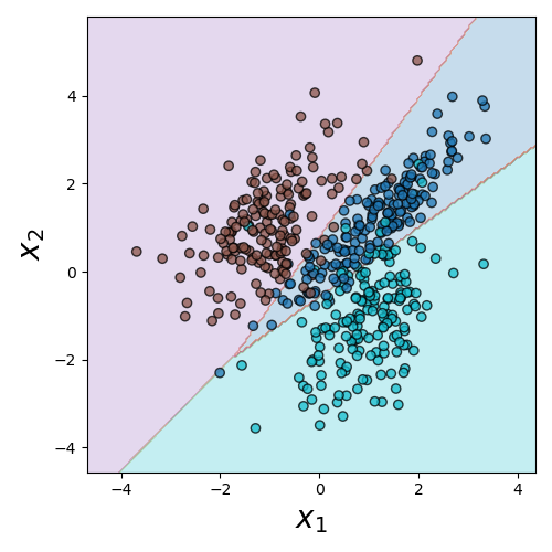
Decision Boundary (Python)
Need to import:
from sklearn.inspection import DecisionBoundaryDisplay as DBDCreate the plot from the estimator:
DBD.from_estimator(model, df[[features]])- Unlike the confusion matrix, here the estimate needs both the model and the feature values to predict from
- Can also pass in other arguments, like axis labels or the actual axis you want to add the plot to
Your Turn!
Activity!
- The dataset here has two independent variables and then a label column that can be one of three options
- Fit a Logistic Multinomial Regression model to the data and compute the resulting confusion matrix and model accuracy