Fitting
Jed Rembold
March 30, 2026
Announcements
- HW10 coming out today
- New unit!
- New partners at the end of today
- Unit 4 debrief form active until the end of the week
- Quiz 2 supposed to be on Wednesday
- I am a bit uncomfortable asking you to do this without at least some feedback from HW on these units
- How would we feel about delaying this a week?
Recap
- Ensemble models can help combat noisy data where a single model tends to overfit the noise
- To be effective, need the individual models to be non-correlated
- Commonly achieved through bootstrap aggregation (bagging)
- Random forests are an ensemble of decision trees
- In addition to bagging, they consider a random subset of features at each decision
- Parameters general concern the size of the forest, the number of features considered, or other pre-pruning options
- General grant the benefits of decision trees, but without the inherent instability
Discussing Today
- What do we want from a model fit?
- Why might we need methods beyond least-mean squares?
- How can randomness help us determine the output of integrals?
Data Fitting
Why fit data?
- A “fit” model computes the values of unknown constants within the model
- In science, and in astronomy in particular, such models are usually
derived from fundamental first principles, and thus those constants are
linked to physical properties or laws
- The
Twhen we fit Planck’s Law, for instance
- The
- Individual fits themselves may still not be that important: rather,
they can contribute to an overall story that the data is telling
- “Hotter things emit more light and bluer light”
Fitting Neglect
- In the fitting that we have done so far this semester, we have been
leaving some important things out
- What role does any known error or variance play in our fitting of data?
- How confident should we be in our fit parameters? That is, what variance should we expect in the fit parameters?
- All of these things can sometimes be estimated easily from
current techniques, and can sometimes have easy analytic
results.
- But what about in more complicated situations?
Case Study: Integration
A seeming aside: Solving Integrals
- Suppose you want to find the area under a function \(f(x)\) between \(x=a\) and \(x=b\), such that you are interested in \[ \int_a^b f(x)\,dx \]
- If \(f(x)\) is simple and you know a bit of calculus, this is relatively straightforward
- But what if \(f(x)\) is some
terribly complicated function that you don’t know how to integrate?
- Or worse, what if \(f(x)\) is a largely black-box, wherein you put in an input and then some time later get an output, without seeing what happens in the middle?
Alternative Approaches
- When posed with an intractable integral, most folks these days look
to:
- Wolfram Alpha, or some other computation engine, for aid with analytic integration
- Numerical techniques
- Numerical techniques rely on breaking the integral up into simple
approximations
- The key here is that they are always approximations (midpoint rule, trapezoid rule, Simpson’s rule, etc.)
- As approximations, there will always be some inherent error associated with using these methods
Entering the Multiverse
- For nice one-dimensional problems, these methods can work out nicely
- But what if our function was instead dependent on, for instance, 6 parameters? \[ f(x,y,z,a,b,c) \quad\rightarrow\quad \int\int\int\int\int\int f(x,y,z,a,b,c)\,dx\,dy\,dz\,da\,db\,dc \]
- The trapezoid rule is a decent approximation method, but if you work it out, its error scales as: \[ \epsilon \propto \frac{1}{N^{2/d}} \] where \(N\) is the number of sample points (how skinny are the rectangles) and \(d\) the number of dimensions being integrated over
Compiling Errors
- In order to keep a constant error value then as the number of dimensions increase: \[ N = (1/\epsilon)^{d/2} \]
- This is highly problematic for higher dimensional data, as we need
exponentially more data to keep the errors at a given level!
- We need to compute the area of each of those trapezoids, so exponentially more trapezoids means exponentially longer running time
A Random Rescue
A Random Solution
- What if, instead of slicing up the entire region of interest, we instead randomly sampled from that region
- Computing, for instance, just the area at a given, randomly selected point
- It turns out this error scales as: \[ \epsilon \propto \frac{1}{\sqrt{N}} \] which no longer has any \(d\) dependence!!
- This is the basis behind random (or Monte Carlo) selection methods
Random Areas?
- How do random points get us an accurate portrayal of the area under
the curve?
- At each random point, compute the value of the function at that point, this will be the height of your rectangle
- The width of your rectangle is just the span of your boundaries
- Some points will overestimate the area, and some will underestimate the area
- The amazing aspect is that given enough points, the average of the point areas will closely approximate the actual area under the curve
Example
Suppose we wanted to evaluate the area under the curve \[ f(x) = -\frac{4}{5}x + 4 \] from \(x=0\) to \(x=5\), using Monte Carlo methods. This describes a triangle with height 4 and width 5, and thus should have an area of 10. Is that what we get?
Example 2
What if we slightly complicate this function by looking instead at a piece-wise function: \[ f(x) = \begin{cases} 0 & 0 \leq x < 2; \\ -\frac{4}{5}x + 3.2 & 2 \leq x \leq 4; \\ 0 & 4 < x \leq 5 \end{cases} \] This now describes a triangle with height of 1.6 and width of 2, thus having an area of 1.6. Does the Monte Carlo method still work?
The Probable
Probability Distributions
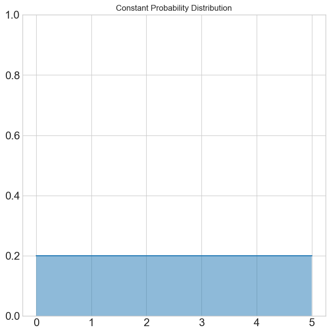
- A probability distribution describes the likelihood of selecting a particular value over a range of values.
- The area under the probability distribution must sum to 1, so the odds add up.
- In our current examples, any number between 0 and 5 was equally likely, which would have led to the probability distribution to the right.
Importance
- For some functions, all points might not be equally interesting, and thus a constant probability distribution makes no sense.
- We instead might want to weigh certain regions higher in our random selection, as that is where the interesting things are happening
- If we do so, we need to recognize that in computing our areas, we
are now doing \[ A = \frac{f(x_k)}{p(x_k)}
\] where \(p(x_k)\) is the
probability of selecting a particular \(x\)
- This is the same as what we were doing before, since for a uniform sampling, the probability weights looked like 0.2, and 1/0.2 is 5.
Selecting from a probability distribution
Selecting discrete values from a continuous probability distribution often utilizes Rejection Sampling
One implementation, in Python, might look like:
def sample_from_prob_dist(pdf, lower, upper, num):
    samples = np.zeros(num)
    count = 0
    while count < num:
        x = np.random.uniform(lower, upper)
        if np.random.uniform(0,1) <= pdf(x):
            samples[count] = x
            count += 1
    return samples
Rejection Sampling in R
- Doing the same thing in R, but pre-allocating the list for better performance:
samp <- function(pdf, lower, upper, num) {
  samples <- numeric(num)
  count <- 0
  while (count < num) {
    x <- runif(1, lower, upper)
    if (runif(1, 0, 1) <= pdf(x)) {
      count <- count + 1
      samples[count] <- x
    }
  }
  return(samples)
}
Example 3
Now suppose we wanted to evaluate the area under the same piece-wise function as earlier: \[ f(x) = \begin{cases} 0 & x < 2; \\ -\frac{4}{5}x + 3.2 & 2 \leq x \leq 4; \\ 0 & x > 4 \end{cases} \] But this time choosing points based on two different probability distributions: \[ {p(x) = \begin{cases} 0 & x < 2; \\ 0.5 & 2 \leq x \leq 4; \\ 0 & x > 4 \end{cases}}\qquad {p(x) = \begin{cases} 0 & x < 2; \\ \frac{1}{2}\left(x - 2\right) & 2 \leq x \leq 4; \\ 0 & x > 4 \end{cases}} \]
An Unknown PDF
- What if we don’t know or have a PDF to work with?
- The perfect PDF would look just like the function we are
trying to integrate, but scaled to have area = 1
- But if we could easily calculate the area, we wouldn’t be doing this integration in the first place
- Instead we will construct a process to semi-randomly “walk” it’s way
around our initial function
- Goal is to have it spend more of its time near “higher” parts of the function
- Then we’ll look at the distribution of where it spent time
Looking to HW10
Groups!
- Cordelia and Morgyn
- Normandy and Kaylee
- Saul and Yumi
- Lev and Deana
- Maiti and Laken
- Aby and Cody
- Florian, Liam, and Rebecca
- KJ and Ben
- Jack and Mac