Fitting

Announcements

• HW5 should hopefully be coming out over the coming weekend
  • Things have been a bit slowed by my travel
• I almost got through HW2 feedback before I left, but not quite. I’m so sorry.
• If my current connection does not allow a decent stream, then I’ll make a recording and post it.
• On Tuesday we will have another remote lecture

Recap

• Rotation or velocity curves measure the speed of orbiting objects as you move outwards from a central body
  • Commonly assume circular or largely circular orbits
  • Generally measured through Doppler shifts
• The shape of a rotation curve tells you about the distribution of material throughout the region
• The rotation curves of galaxies do not match what we would expect, thus leading to conjectures about dark matter

Discussing Today

• What do we want from a model fit?
• Why might we need methods beyond least-mean squares?
• How can randomness help us determine the output of integrals?

Why fit data?

• A “fit” model computes the values of unknown constants within the model
• In science, and in astronomy in particular, such models are usually derived from fundamental first principles, and thus those constants are linked to physical properties or laws
  • The T when we fit Planck’s Law, for instance
• Individual fits themselves may still not be that important: rather, they can contribute to an overall story that the data is telling
  • “Hotter things emit more light and bluer light”

Fitting Neglect

• In the fitting that we have done so far this semester, we have been leaving some important things out
  • What role does any known error or variance play in our fitting of data?
  • How confident should we be in our fit parameters? That is, what variance should we expect in the fit parameters?
• All of these things can sometimes be estimated easily from current techniques, and can sometimes have easy analytic results.
  • But what about in more complicated situations?

A seeming aside: Solving Integrals

• Suppose you want to find the area under a function \(f(x)\) between \(x=a\) and \(x=b\), such that you are interested in \[ \int_a^b f(x)\,dx \]
• If \(f(x)\) is simple and you know a bit of calculus, this is relatively straightforward
• But what if \(f(x)\) is some terribly complicated function that you don’t know how to integrate?
  • Or worse, what if \(f(x)\) is a largely black-box, wherein you put in an input and then some time later get an output, without seeing what happens in the middle?

Alternative Approaches

• When posed with an intractable integral, most folks these days look to:
  • Wolfram Alpha, or some other computation engine, for aid with analytic integration
  • Numerical techniques
• Numerical techniques rely on breaking the integral up into simple approximations
  • The key here is that they are always approximations (midpoint rule, trapezoid rule, Simpson’s rule, etc.)
  • As approximations, there will always be some inherent error associated with using these methods

Entering the Multiverse

• For nice one-dimensional problems, these methods can work out nicely
• But what if our function was instead dependent on, for instance, 6 parameters? \[ f(x,y,z,a,b,c) \quad\rightarrow\quad \int\int\int\int\int\int f(x,y,z,a,b,c)\,dx\,dy\,dz\,da\,db\,dc \]
• The trapezoid rule is a decent approximation method, but if you work it out, its error scales as: \[ \epsilon \propto \frac{1}{N^{2/d}} \] where \(N\) is the number of sample points (how skinny are the rectangles) and \(d\) the number of dimensions being integrated over

Compiling Errors

• In order to keep a constant error value then as the number of dimensions increase: \[ N = (1/\epsilon)^{d/2} \]
• This is highly problematic for higher dimensional data, as we need exponentially more data to keep the errors at a given level!
  • We need to compute the area of each of those trapezoids, so exponentially more trapezoids means exponentially longer running time

A Random Solution

• What if, instead of slicing up the entire region of interest, we instead randomly sampled from that region
• Computing, for instance, just the area at a given, randomly selected point
• It turns out this error scales as: \[ \epsilon \propto \frac{1}{\sqrt{N}} \] which no longer has any \(d\) dependence!!
• This is the basis behind random (or Monte Carlo) selection methods

Random Areas?

• How do random points get us an accurate portrayal of the area under the curve?
  • At each random point, compute the value of the function at that point, this will be the height of your rectangle
  • The width of your rectangle is just the span of your boundaries
• Some points will overestimate the area, and some will underestimate the area
• The amazing aspect is that given enough points, the average of the point areas will closely approximate the actual area under the curve

Example

Suppose we wanted to evaluate the area under the curve \[ f(x) = -\frac{4}{5}x + 4 \] from \(x=0\) to \(x=5\), using Monte Carlo methods. This describes a triangle with height 4 and width 5, and thus should have an area of 20. Is that what we get?

Example 2

What if we slightly complicate this function by looking instead at a piece-wise function: \[ f(x) = \begin{cases} 0 & x < 3; \\ -\frac{4}{5}x + 4 & 3 \leq x \leq 5; \\ 0 & x > 5 \end{cases} \] This now describes a triangle with height of 1.6 and width of 2, thus having an area of 1.6. Does the Monte Carlo method still work?

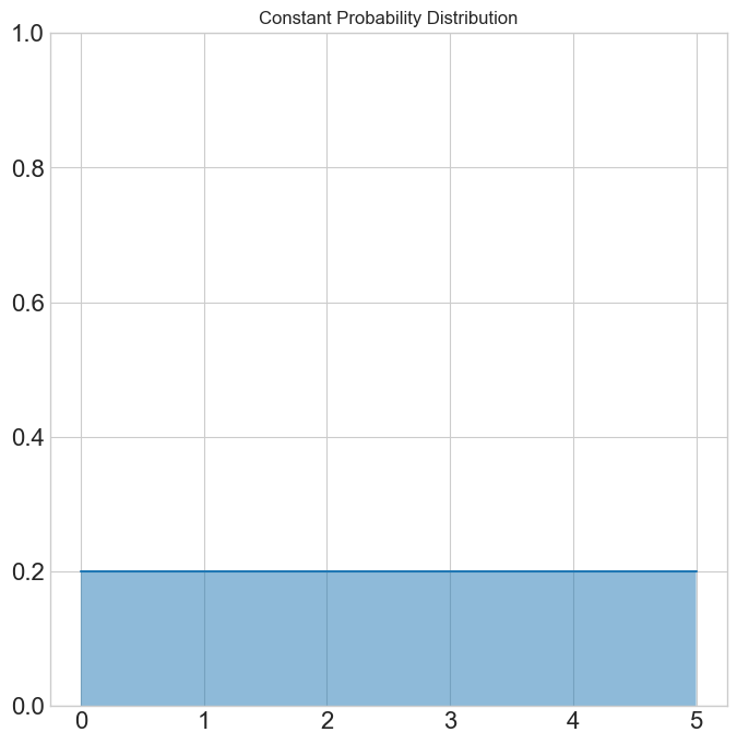
Probability Distributions

Importance

• For some functions, all points might not be equally interesting, and thus a constant probability distribution makes no sense.
• We instead might want to weigh certain regions higher in our random selection, as that is where the interesting things are happening
• If we do so, we need to recognize that in computing our areas, we are now doing \[ A = \frac{f(x_k)}{p(x_k)} \] where \(p(x_k)\) is the probability of selecting a particular \(x\)
  • This is the same as what we were doing before, since for a uniform sampling, the probability weights looked like 0.2, and 1/0.2 is 5.

Selecting from a probability distribution

• Trying to select from a continuous probability distribution discretely is not ideal, but that is all that is immediately available through Numpy

• For a better option, roll your own selector:

  def sample_from_prob_dist(pdf, lower, upper, num):
      samples = []
      while len(samples) < num:
          x = np.random.uniform(lower, upper)
          p = pdf(x)
          if np.random.uniform(0,1) <= p:
              samples.append(x)
      return np.array(samples)

Example 3

Now suppose we wanted to evaluate the area under the same piece-wise function as earlier: \[ f(x) = \begin{cases} 0 & x < 3; \\ -\frac{4}{5}x + 4 & 3 \leq x \leq 5; \\ 0 & x > 5 \end{cases} \] But this time choosing points based on two different probability distributions: \[ {p(x) = \begin{cases} 0 & x < 3; \\ 0.5 & 3 \leq x \leq 5; \\ 0 & x > 5 \end{cases}}\qquad {p(x) = \begin{cases} 0 & x < 3; \\ \frac{1}{2}\left(x - 3\right) & 3 \leq x \leq 5; \\ 0 & x > 5 \end{cases}} \]

An Unknown PDF

• What if we don’t know or have a PDF to work with?
• The perfect PDF would look just like the function we are trying to integrate, but scaled to have area = 1
  • But if we could easily calculate the area, we wouldn’t be doing this integration in the first place
• Instead we will construct a Markov Chain to semi-randomly “walk” it’s way around our initial function
  • Goal is to have it spend more of its time near “higher” parts of the function
  • Then we’ll look at the distribution of where it spent time

Markov Chains

• A Markov chain is a model that represents a sequence of events where the probability of the next event is determined only by the current event
• In our case, the point we are currently “at” will make it likely that our next point is nearby
• Our process will then follow that of Metropolis-Hastings and is shown below. Note that you must keep track of the visited points along the way!
  • Choose a starting point
  • For some number of iterations:
    • Randomly choose a nearby point
    • Compare that point to your current point, to see if it would move you “higher” up the function
    • If above a random threshold, move to that point, otherwise stay where you are at

Choosing a Nearby Point

• Randomly choosing a nearby point inherently pulls from a probability distribution centered on the current point

• Most frequently used is a Gaussian probability distribution

  • Centered (mean) on the current point
  • Spread (std) can be tuned, but 1 is a reasonable starting value

  np.random.normal(loc=0, spread=1)

• Working in higher dimensions? A multi-variate Gaussian will still work!

  np.random.multivariate_normal(mean=VEC, cov=MAT)

Move onward or stay?

• Once you have the new point candidate, you need to decide whether to keep it or your current point
• In Metropolis-Hastings, you:
  • Take the ratio of your sampled function evaluated at the new point over the sampled function evaluated at the current \[ \frac{f(x^\prime)}{f(x)} \] where \(x\) is your current position and \(x^\prime\) your proposed new position
  • Compare that ratio to a randomly generated number between 0 and 1
    • If bigger, keep the new position, making it your new current
    • If smaller, keep the old position (but still add it to your visited list again)

Backing out a PDF

• The history of the random walk contains information about where the walker spent the most time
  • Due to how we constructed the walk, this should be near the maximum portions of our function
• Creating a histogram or KDE plot will allow us to visualize the probability distribution.
• We could use the histogram information to directly sample from the distribution