Markov Chains

• A Markov chain is a model that represents a sequence of events where the probability of the next event is determined only by the current event
• In our case, the point we are currently “at” will make it likely that our next point is nearby
  • However, we don’t just want a totally random nearby point
• We want to generally walk “uphill”, because that’s where the important “stuff” is, but we don’t want to always go uphill
  • Why not?
    • We could get “stuck” in a local maximum
    • Our whole goal is to “sample” the space, not directly optimize it. A bit of wandering is a good thing!

Metropolis-Hastings

• There are a variety of potential algorithms, but we’ll follow the work of Metropolis and Hastings
• Our process will be as follows:
  1. Start a list of all the visited points (initially empty)
  2. Choose a starting point, and add it to the visited list
  3. For some number of iterations:
     • Randomly choose point nearby to your current location
     • Compare that point to your current point, to see if it would move you “higher” up the function
     • Randomly select a number and compare to a threshold. If the number is smaller, move to that point, otherwise revisit your current location.
       • Add your destination to your visited list

Taking a Step

• Randomly choosing a nearby point inherently pulls from a probability distribution centered on the current point
• Most frequently used is a Gaussian probability distribution
  • Centered (mean) on the current point
  • Spread (std) can be tuned, but 1 is a reasonable starting value
    • Smaller values equate to smaller steps, bigger values to potentially bigger steps

  np.random.normal(mean, std, num)

  rnorm(num, mean, std)

Higher Dimensional Steps

• Working in higher dimensions? A multivariate Gaussian will still work!

  np.random.multivariate_normal(mean=VEC, cov=MAT)

  MASS::mvrnorm(n, mu=VEC, Sigma=MAT)

• The diagonal elements of MAT are your \(\sigma^2\) values for each dimension

  • You might just be able to use the identity matrix for some situations, but in other cases you might want to make very different step sizes in different directions

Move onward or stay?

• Once you have the new point, you need to decide whether to keep it or your current point
• In the Metropolis-Hastings algorithm, you:
  • Take the ratio of your sampled function evaluated at the new point over the sampled function evaluated at the current \[ \frac{f(x^\prime)}{f(x)} \] where \(x\) is your current position and \(x^\prime\) your proposed new position
  • Compare that ratio to a randomly generated number between 0 and 1
    • If the ratio is bigger, keep the new position, making it your new current
    • If the ratio is smaller, keep the old position (but still add it to your visited list again)

Hand Example

Backing out a PDF

• The history of the random walk contains information about where the walker spent the most time
  • Due to how we constructed the walk, this should be near the maximum portions of our function
• Creating a histogram or KDE plot will allow us to visualize the probability distribution.
• We could use the histogram information to directly sample from the distribution

Example: Walking the Function

• Last class we were looking at the piece-wise function described by: \[ f(x) = \begin{cases} 0 & x < 2; \\ -\frac{4}{5}x + 3.2 & 2 \leq x \leq 4; \\ 0 & x > 4 \end{cases} \]
• Let’s “walk” this function according to Metropolis-Hastings to generate a PDF of the same shape

Check Yourself

• Just because your MCMC sampler ran to completion does not mean you got good results!
  • If your steps were too small or too large, you might not have “discovered” everything there is to discover
  • If your starting position was far from anything interesting, your sampler might still be walking constantly uphill
• We need ways to check for these things, and then potentially re-evaluate our sampler

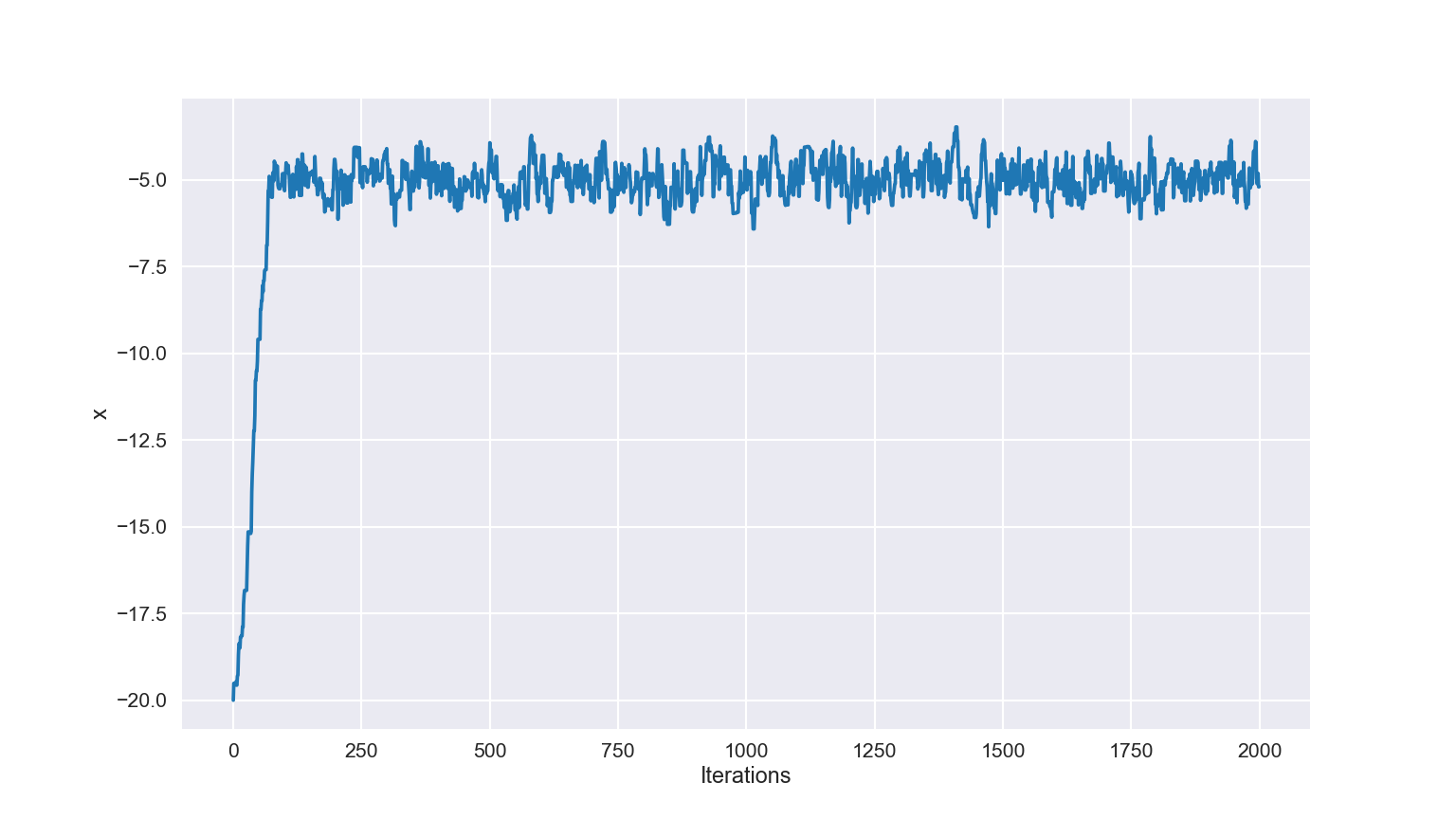
Trace Plots

• Because our starting point is often just a random guess, it might take time for the sampler to travel to anything interesting
• Usually, we do not care about this part of the chain
• Can view this with a Trace Plot, where we plot the iteration number against the parameter value
• Looking for a “hairy caterpillar”, where the parameter eventually settles down to jumping about a region
• Remove the earlier region, leaving just the burned-in sampled data

Example Trace

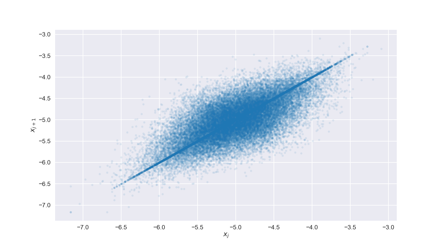
Lag Plots

• If our steps are too small or too large, we can fail to adequately sample the function
  • Too small, and we don’t actually travel anywhere
  • Too big, and we can reject too many steps, making us stay in the same place for long periods of time
• Ideally, we want each step to be as independent of the previous position as possible
• A Lag Plot, where we plot a parameters current position against its next position can help showcase this
  • If everything shows up on a diagonal line, that is bad. The walker either isn’t moving or is barely moving
  • If we get a nice blobby cloud, that is good!

Lag Example

Gaining Acceptance

• The Acceptance Rate is the percentage of proposed steps that are accepted
• Too high or too low is bad, as it implies either:
  • Your walker has yet to find the region of interest
  • Your walker rarely moves
• For 1D data, a rate of around 40-50% often gives decent results
• For higher dimensional data, that is closer to 20-30%

Your Turn

• Download a simple library (Python or R) that contains a function called mystery, which accepts a single parameter x
• Your task is to thoroughly sample the unknown function using MCMC
  • Choose a starting point
  • Choose a step size
  • Run it
  • Diagnose your results
• Compare to your neighbors! Different chains can reveal more about a function!