Model Fitting and Baye’s Theorem

• Here we are not as concerned with the best fit
• Concerned instead with our confidence about our fit parameters
  • “What was the probability of getting these parameters given this data?”
• Baye’s Theorem provides a way to compute this probability \[ P(\theta | D) = \frac{P(D | \theta) \cdot P(\theta)}{P(D)} \] where \(\theta\) represents our fit parameters and \(D\) represents the data
• For our purposes, viewing this through a Bayesian lens will be more informative

Baye Life

The Breakdown (Part I)

• The Prior is the probability of the parameters without any consideration of the data
  • This generally reflects any knowns or assumptions you are making about the parameters
  • Are they all positive? Are they bounded in some way?
• The Likelihood is the probability of getting the data given the parameters
  • For model fitting, this is where we compare the actual data to the predicted data by our model
  • The better the match, the greater the likelihood

The Breakdown (Part II)

• The Evidence is the probability of the data being the way it is
  • This is extremely hard to measure, and also largely pointless for our use-case
  • It doesn’t depend on the parameters, so would just be a constant scaling factor
• The Posterior is the probability of the parameters given the data
  • This is what we want!
  • “How likely are these parameters given our data?”

The Big Picture

• Our goal here is to sample the right-hand side of Baye’s theorem using MCMC
• The resulting distribution would also describe the probabilities on the left-hand side
  • At least within a scaling factor
• What we are really interested in though is the spread of the posterior probability distribution, so this scaling is of no consequence to us

Logging

• We can get a pretty huge dynamic range when computing the values of the right-hand side
• Recall that we compute these for each step to see if we take the random step or not
• To avoid computational overflow/underflow errors, it can be recommended to work in ln-space instead
• Here, the accept/rejection step becomes: \[\frac{f(\theta^\prime)}{f(\theta)} > r \quad\rightarrow\quad \ln f(\theta^\prime) - \ln f(\theta) > \ln r \]

The Prior

• The prior dictates the probability of a parameter having a particular value, regardless of the data

• If using an unbounded, flat, prior, then it should just return 1 always (0 in ln-space)

• If bounded, check the parameters and return 1 (0 in ln-space) if within the bounds or \(-\infty\) otherwise (-np.inf in Python, -Inf in R)

• Pseudo-example:

  |||function ln_prior(|||params|||)|||
    if |||illegal condition|||
      return -|||infinity|||
    return 0

  |||function ln_prior(|||params|||)|||
    if |||legal condition|||
      return 0
    return -|||infinity|||

The Likelihood

• The likelihood essentially compares the data our model would output to our actual data
• The goal is to minimize the differences between the two
  • Additionally, things are normally scaled by known errors, so that values with more error have less weight
• If our individual data points were arranged around the model with some uncertainty: \[ P(y_i | \theta,\sigma) = \frac{1}{\sqrt{2\pi\sigma^2}} \exp\left(-\frac{(y_i - f(x_i, \theta))^2}{2\sigma^2}\right)\]
• The likelihood is just the sum over all these points. So \[ \log \mathcal{L} = \sum^n_{i=1}\log P(y_i|\theta,\sigma) = \sum^n_{i=1}\left[ -\frac{(y_i - f(x_i,\theta))^2}{2\sigma^2}-\frac{1}{2}\log(2\pi\sigma^2)\right]\]

The Likelihood (In Code)

• The ln-likelihood then could look like:

  |||function ln_likelihood(|||params, data|||)|||
    m,b = params
    x,y,errY = data # extract data
    y_model = m * x + b # compute model result
    residual = y - y_model # compute the difference
    term1 = - 0.5 * |||log|||(2 * |||pi||| * errY ** 2)
    term2 = - 0.5 * (y - y_model) ** 2 / errY ** 2 )
    return |||sum|||(term1 + term2)

All together now…

• Bring both pieces together (since we don’t care about \(P(D)\)):

  |||function ln_pdf(|||params, data|||)|||
    p = |||call ln_prior|||
    if p == -|||infinity||| # no sense continuing
      return -|||infinity|||
    return p + ln_likelihood(params, data)

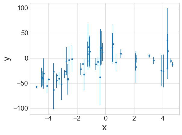
Extended Example

Reminder!

• All previous methods still hold:
  • Trace plots to establish that things have leveled off and determine potential burn-in
  • Lag plots to investigate if your step-sizes looked good
  • Histograms to visualize the spread of the parameters
    • For higher dimensional fits, pair-wise 2d histograms are very common

Visualizing the Best Fit with Errors

• There are a few ways you can visualize the best fit model with uncertainties in the parameters reflected
• My go-to looks like:
  • Randomly select some number of indices from your leveled chain
  • For each index, grab the corresponding parameters and compute your model output with those parameters, appending the result to a list
  • Compute the median and standard deviation of the results in your list, being sure to specify axis=0
  • Plot the median values for your best approximation, and shade the region between the median - std and the median + std
• Alternatively, you could just plot the model output for each of the randomly selected parameter combinations, though I don’t think it looks as nice