Available Options

• While it isn’t difficult to create our own MCMC sampler, there can be some benefits to using existing libraries for more complicated use cases
  • Tend to give more intuitive interfaces through which to accomplish the basic tasks that we would want
• In the Python landscape, the main option used is the emcee package, which you will probably need to install through pip
  • Emcee operates as an abstract data type, wherein you create a sampling object and then can interact with it and run samples using defined methods
• In the R landscape, I recently discovered the mcmcensemble library, which seems to be the closest analog to Python’s emcee

Python: Emcee Creation

• When you create the object initially, you need to provide:
  • The number of walkers you’d like to generate
  • The number of dimensions you’ll be walking (number of parameters)
  • The function you’ll be walking (your log posterior)
  • Any extra arguments that your function will need beyond the parameters
  • A pool should you be using multiprocessing

  sampler = emcee.EnsembleSampler(
                num_walkers, num_dims,
                log_function, args=[extra arguments]
                )

Python: Emcee Running

• Generating starting points usually done with some variation of a random gaussian near a starting point:

  starts = np.random.multivariate_normal(
              mean = [0,1,10],
              cov = [[1,0,0],[0,0.5,0], [0,0,5]],
              size = num_walkers
              )

• You can then start a sampling run by telling the sampler where all the walkers should begin and how many steps they should take

  sampler.run_mcmc(starts, num_iterations)

Python: Emcee Retrieving Chains

• You can get the iteration chains back from the sampler after a run using .get_chain()

  • This will usually return a 3D array, indexing over the parameter, walker, and iteration

  • Can visualize a particular parameter over all walkers using

    plt.plot(sampler.get_chain()[:,:,0], 'k', alpha=0.3)

• After examining, will commonly want to discard the burn in and flatten all the individual walkers:

  flat_samples = sampler.get_chain(discard=num_dis, 
                                   flat=True)

Python: Interpreting Results

• Commonly several things you’ll want to look at after flattening the chains:
  • Histograms of the individual parameter distributions
  • 2D Histograms/KDE plots of pair-wise parameter combinations
  • Visualizing the best fit with errors back on the original dataset
• The first two can be done individually, or they can be streamlined using the corner package
  • corner will automatically generate both individual parameter distributions and all pair-wise 2D histograms

R: MCMC Ensemble

• Need to install and load the mcmcensemble package and the bayesplot package for nicer plotting

• Can specify multiple starting points for walkers in a similar way to in Python:

  p_means <- c(0, 1, 10)
  p_cov <- matrix(c(1, 0, 0, 0, 0.5, 0, 0, 0, 5), 3)
  starts <- MASS::mvrnorm(
    n=n_walkers, mu=p_means, Sigma=p_cov
  )

R: Running the Walker

• To actually generate the samples, you do:

  sampler <- MCMCEnsemble(
        f = ln_pdf,            # The function you are walking
        inits=walker_starts,   # Where each walker starts
        max.iter = 1000*30,    # The total number of steps
        n.walkers=n_walkers,   # The number of walkers
        coda=TRUE              # Format output nicely
  )

• You can trim to remove burn-in with:

  burned <- window(sampler$samples, start=500)

R: Visualizing Results

• The bayesplot library gives you lots of easy ways to visualize CODA formatted walker chains
• Trace plots: mcmc_trace(sampler$samples)
• Histograms: mcmc_hist(sampler$samples)
• KDE plots: mcmc_dens(sampler$samples)
• Summary stats: summary(sampler$samples)

R: One More

• One more library that you may find useful is ggmcmc

• Allows you to convert your sampler$samples into a nice dataframe easily:

  samples <- ggs(sampler$samples)

• Then lots of visualizing functions that dataframe can be passed into:

  • ggs_traceplot(samples)
  • ggs_pairs(samples)
  • ggs_histogram(samples)

Circular Speeds

Velocity Dependence

• We can work out how the velocity should vary with distance from the center: \[\begin{aligned} F_{grav} &= \frac{mv_{circ}^2}{R}\\ \frac{GMm}{R^2} &= \frac{mv_{circ}^2}{R}\\ \frac{GM}{R} &= v_{circ}^2 \end{aligned} \]
• For nicely symmetric mass distributions, \(M\) can be taken to be the total mass internal to the radius \(R\) \[ v_{circ}(R) = \sqrt{\frac{GM_{in}(R)}{R}} \]

Consistent Mass

Consistent Density

Quiz 2

• You know the drill
• The rest of class today is set aside for Quiz 2 on exoplanets and galaxies
• You are free to leave when you are done!

Visualizing Rotations

Activity

• I am providing you with two density profiles below:
  • Solar System-like (density in \(kg/au^3\))
  • Galaxy-like (density in \(kg/ly^3\))
• For each, you can assume that the density beside a distance describes the density between that distance and the previous distance
• You task is to generate velocity curve profiles for each. You can assume a spherical distribution of the material.
• How do they compare (both to one another and the distributions we just looked at)?

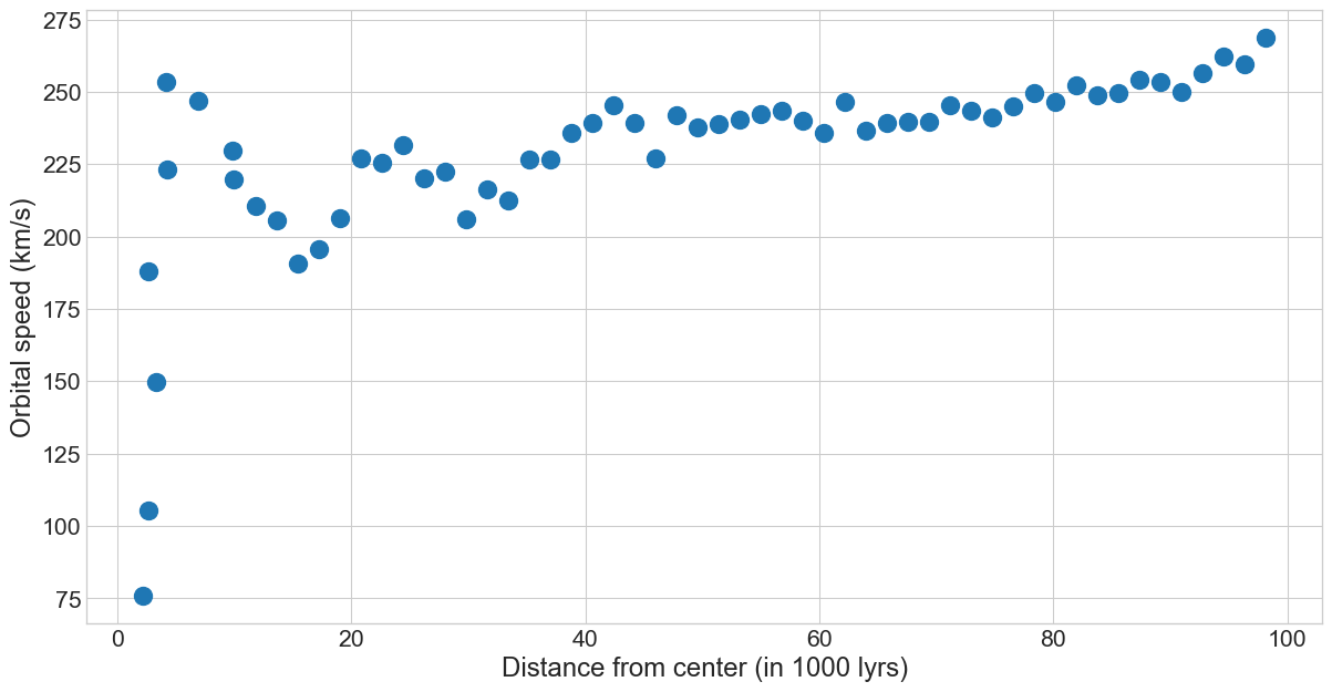
Surprises

• The second velocity curve is what astronomers expected to see when looking at the Milky Way and other galaxies
  • Would be consistent with the visible light we saw from the galaxy and known star masses
• But instead…

Rotation Curve: Milky Way

Rotation Curve: Others

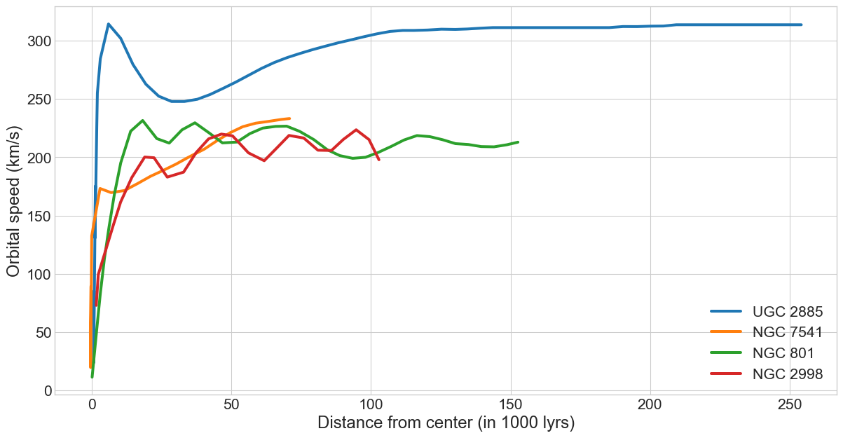
Possibilities

• Determining how to reconcile the mass that we see, with the mass that the rotation curves predict, has been an ongoing struggle
• Current estimates predict between 5-10 times as much mass as we see
  • Spread somewhat evenly throughout the visible galaxy and far beyond
• Definitely does not seem to have the majority of mass concentrated at the center
• Are we missing dark objects?

Being MACHO

• What other forms of mass do we know of that would be faint / invisible?
• Could the halo of the galaxy be filled with faint, dead stars?
  • Massive Compact Halo Objects?
  • Brown dwarfs
  • Neutron stars
  • Black Holes
• How does one find an invisible object?

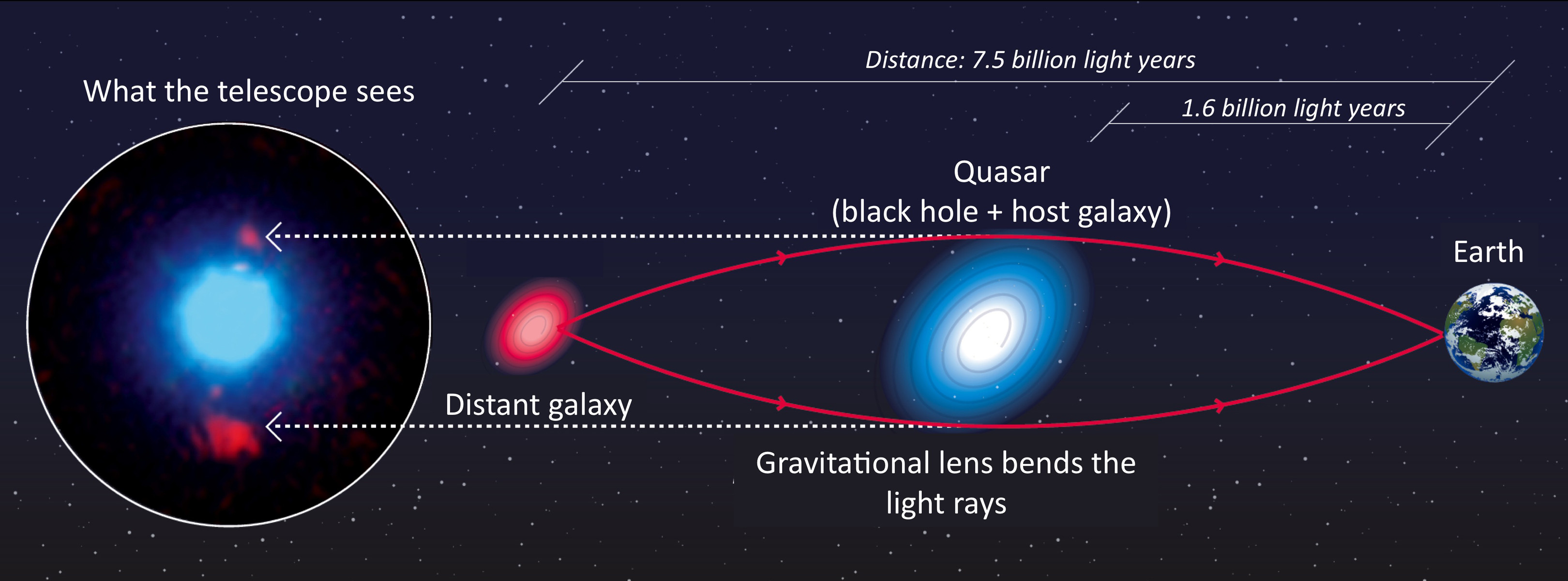
Gravitational (Micro)Lensing

• We look for their mass’s effect on nearby light
• Find that MACHO’s account for maybe 20% of the missing mass, at most
• Hence, the currently named dark matter