---
title: "Does Dark Matter?"
author: Jed Rembold
date: April 15, 2025
slideNumber: true
theme: tokyo-night-light
highlightjs-theme: tokyo-night-light
width: 1920
height: 1080
transition: fade
p5js: true
---
## Announcements
- HW5 was due! Try to get it in soon if you are a bit behind, as HW6 (the last one) is coming out soon!
- HW5 Debrief becomes available at midnight tonight through Thursday at midnight
- Quiz 2 scores will be handed back on Thursday
- My end of week and weekend was very full, so the group preferences poll didn't get posted. Expect that tonight.
## Recap
- A Monte Carlo Markov Chain is a semi-random walk wherein the next step is determined by the current location and a bit of randomness
- Directed in the sense that is has a preference to move "uphill", toward higher parts of the function it is sampling
- We can sample the probability of parameters given particular data ($P(\theta | D)$) using Baye's theorem
- Requires being able to write out our priors and our likelihood
## Discussing Today
- Libraries for MCMC
- What is dark matter?
- Why do we think it exists?
- How can we measure it?
- What ramifications does it have?
# Helpful MCMC Libraries
## Available Options
- While it isn't difficult to create our own MCMC sampler, there can be some benefits to using existing libraries for more complicated use cases
- Tend to give more intuitive interfaces through which to accomplish the basic tasks that we would want
- In the Python landscape, the main option used is the `emcee` package, which you will probably need to install through `pip`
- `Emcee` operates as an abstract data type, wherein you create a sampling object and then can interact with it and run samples using defined methods
- In the R landscape, there is the `mcmc` package, which also seems reasonably strong, though it doesn't seem to have all of the flexibility of `emcee`
## Python: Emcee Creation
- When you create the object initially, you need to provide:
- The number of walkers you'd like to generate
- The number of dimensions you'll be walking (number of parameters)
- The function you'll be walking (your log posterior)
- Any extra arguments that your function will need beyond the parameters
- A pool should you be using multiprocessing
```python
sampler = emcee.EnsembleSampler(
num_walkers, num_dims,
log_function, args=[extra arguments]
)
```
## Python: Emcee Running
- Generating starting points usually done with some variation of a random gaussian near a starting point:
```python
starts = np.random.multivariate_normal(
mean = [0,1,10],
cov = [[1,0,0],[0,0.5,0], [0,0,5]],
size = num_walkers
)
```
- You can then start a sampling run by telling the sampler where all the walkers should begin and how many steps they should take
```python
sampler.run_mcmc(starts, num_iterations)
```
## Python: Emcee Retrieving Chains
- You can get the iteration chains back from the sampler after a run using `.get_chain()`
- This will usually return a 3D array, indexing over the parameter, walker, and iteration
- Can visualize a particular parameter over all walkers using
```python
plt.plot(sampler.get_chain()[:,:,0], 'k', alpha=0.3)
```
- After examining, will commonly want to discard the burn in and flatten all the individual walkers:
```python
flat_samples = sampler.get_chain(discard=num_dis,
flat=True)
```
## Python: Interpreting Results
- Commonly several things you'll want to look at after flattening the chains:
- Histograms of the individual parameter distributions
- 2D Histograms/KDE plots of pair-wise parameter combinations
- Visualizing the best fit with errors back on the original dataset
- The first two can be done individually, or they can be streamlined using the `corner` package
- `corner` will automatically generate both individual parameter distributions and all pair-wise 2D histograms
## R: MCMC
- Need to install and load the `mcmc` package
- Gives you the `metrop` function, for Metropolis-Hastings
```r
out <- metrop(ln_pdf, start, num_iterations)
```
- You can then access the chain under: `out$batch`{.r}
- The documentation specifies you want an accepted ratio of around 0.2
- Can use the `scale` argument to adjust this (above 1 is bigger steps, smaller than 1 is smaller steps)
# Why Dark Matter?
## Circular Speeds
::::::cols
::::col
- Objects traveling in a circle need a force pulling them inwards
- The amount of force, size of the circle, and speed are related:
$$ F_{in} = \frac{mv_{circ}^2}{R} $$
- For our orbits, the force must be gravity
::::
::::col
\begin{tikzpicture}%%width=80%
\draw[dashed, very thick] (0,0) circle (3cm);
\draw[-stealth, very thick] (45:3cm) -- + (225:2cm) node[above left] {$\vec F$};
\draw[-stealth, very thick, color=Blue] (45:3cm) -- + (135:1.5cm) node[above right] {$\vec v$};
\draw[thick, fill=Red] (45:3cm) circle (0.5cm);
\end{tikzpicture}
::::
::::::
## Velocity Dependence
- We can work out how the velocity should vary with distance from the center:
$$\begin{aligned}
F_{grav} &= \frac{mv_{circ}^2}{R}\\
\frac{GMm}{R^2} &= \frac{mv_{circ}^2}{R}\\
\frac{GM}{R} &= v_{circ}^2
\end{aligned} $$
- For nicely symmetric mass distributions, $M$ can be taken to be the total mass internal to the radius $R$
$$ v_{circ}(R) = \sqrt{\frac{GM_{in}(R)}{R}} $$
## Consistent Mass
::::::{.cols style='align-items: start'}
::::col
- Consider the mass distribution to the right
- How would the resulting velocity curve look as you moved away from the center?
::::
::::col
\begin{tikzpicture}%%width=100%
\begin{axis}[ybar, bar width=1, xmin=0, xmax=5, ymin=0, ymax=5, xlabel= Distance from Center, ylabel=Mass in region]
\addplot[fill=Purple] coordinates {
(0.5,3) (1.5,3) (2.5,3) (3.5,3) (4.5,3)
};
\end{axis}
\end{tikzpicture}
::::
::::::
## Consistent Density
::::::{.cols style='align-items: start'}
::::col
- Consider instead the spherically symmetric density distribution to the right
- How would the resulting velocity curve look as you moved away from the center?
::::
::::col
\begin{tikzpicture}%%width=100%
\begin{axis}[ybar, bar width=1, xmin=0, xmax=5, ymin=0, ymax=5, xlabel= Distance from Center, ylabel=Density in region]
\addplot[fill=Green] coordinates {
(0.5,3) (1.5,3) (2.5,3) (3.5,3) (4.5,3)
};
\end{axis}
\end{tikzpicture}
::::
::::::
## Visualizing Rotations
## Activity
- I am providing you with two _density_ profiles below:
- [Solar System-like](../demos/L19_solar.csv) (density in $kg/au^3$)
- [Galaxy-like](../demos/L19_galaxy.csv) (density in $kg/ly^3$)
- For each, you can assume that the density beside a distance describes the density between that distance and the _previous_ distance
- You task is to generate velocity curve profiles for each. You can assume a spherical distribution of the material.
- How do they compare (both to one another and the distributions we just looked at)?
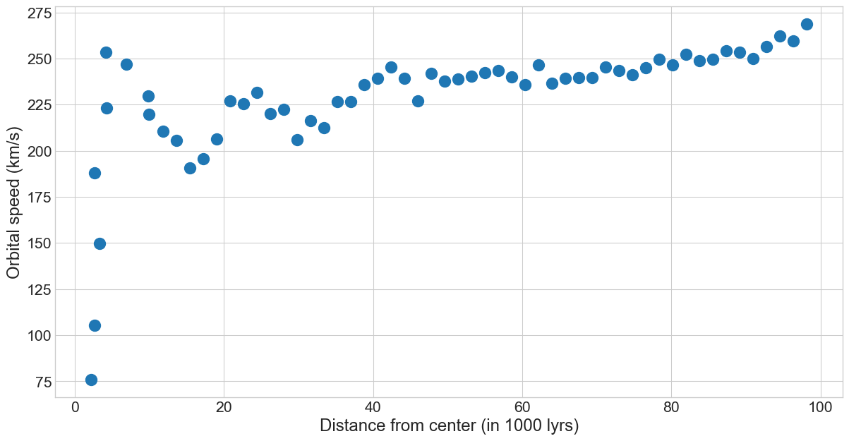
## Surprises
- The second velocity curve is what astronomers expected to see when looking at the Milky Way and other galaxies
- Would be consistent with the visible light we saw from the galaxy and known star masses
- But instead...
## Rotation Curve: Milky Way
{width=100%}
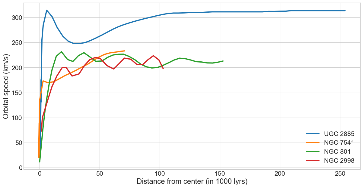
## Rotation Curve: Others
{width=100%}
## Possibilities
- Determining how to reconcile the mass that we **see**, with the mass that the rotation curves predict, has been an ongoing struggle
- Current estimates predict between 5-10 times as much mass as we see
- Spread somewhat evenly throughout the visible galaxy and far beyond
- Definitely does **not** seem to have the majority of mass concentrated at the center
- Are we missing dark objects?
## Being MACHO
- What other forms of mass do we know of that would be faint / invisible?
- Could the halo of the galaxy be filled with faint, dead stars?
- Massive Compact Halo Objects?
- Brown dwarfs
- Neutron stars
- Black Holes
- How does one find an invisible object?
## Gravitational (Micro)Lensing
- We look for their mass's effect on nearby light
- Find that MACHO's account for maybe 20% of the missing mass, at most
- Hence, the currently named _dark matter_
{width=70%}