The Source of Types and Commerce
Jed Rembold
January 22, 2025
Announcements
- Did the first HW get submitted ok?
- If you had any issues, let’s get them figured out before you leave tonight
- My apologies about the Canvas mistake
- Homework 2 is posted! On both the website and Canvas!
- For next week:
- DeBarros: Ch 6
System Objectives
The Primary Objective(s)
There are three main concerns when building any data system:
- Reliability:
- The system works and is not prone to breakage
- Scalability:
- The system can grow as needs or data grows
- Maintainability:
- Future work on the system can be done productively
Secondary Objective
- There are other high-level issues to consider as well
- How do you ensure that the data remains correct and complete?
- How do you handle increased size or data load?
- How should your database interface with users?
- How will you handle errors or problems and the resulting downtime?
External Factors
- Oftentimes “outside” factors can also influence how your system can
be build or managed
- The skill and experience of developers and users
- Any legacy system dependencies
- Time-scale for delivery
- Your organization’s tolerance for risk
- Regulatory climate
Reliability
Reliability
- The system should continue to work correctly, even when
things go wrong.
- The application should perform as the user expects
- The application has a reasonable tolerance for errors or unexpected use
- The application achieves the goals of the use case(s)
- The application prevents abuse or unauthorized access
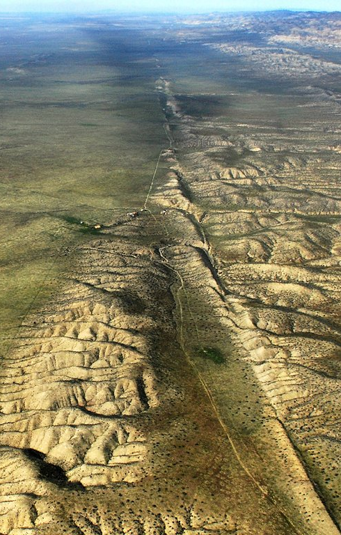
System Resilience
- A fault is anything that could go wrong in the use of a
data system
- Don’t necessarily have to break the entire system (system failure)
- A system that can tolerate faults without entirely breaking is said to be resilient
- Faults are going to happen! The goal is to gracefully handle them and prevent system failure.
- You can not fully plan/mitigate every potential fault
- At some point, you have to accept that the odds of some faults occurring are not worth the expense it would take to mitigate against them.
Fault Types!
- Hardware faults:
-
- Not if, but when hardware will die!
- Software faults:
-
- Probably less likely, but potentially more devastating, as they tend to cascade.
- Human faults:
-
- Potentially the most common source
- Can be managed through careful planning and clear communication
Scalability
Scalability

- As the demands on the data system grow, there should be reasonable
options available for handling the increased demand.
- Understanding exactly how a system’s demands might grow is usually impossible, but the idea is to have contingencies in place and routes where growth COULD happen.
- “If we grow in this way, what options would we have?”
- Requires being able to quantify when the system needs to grow!
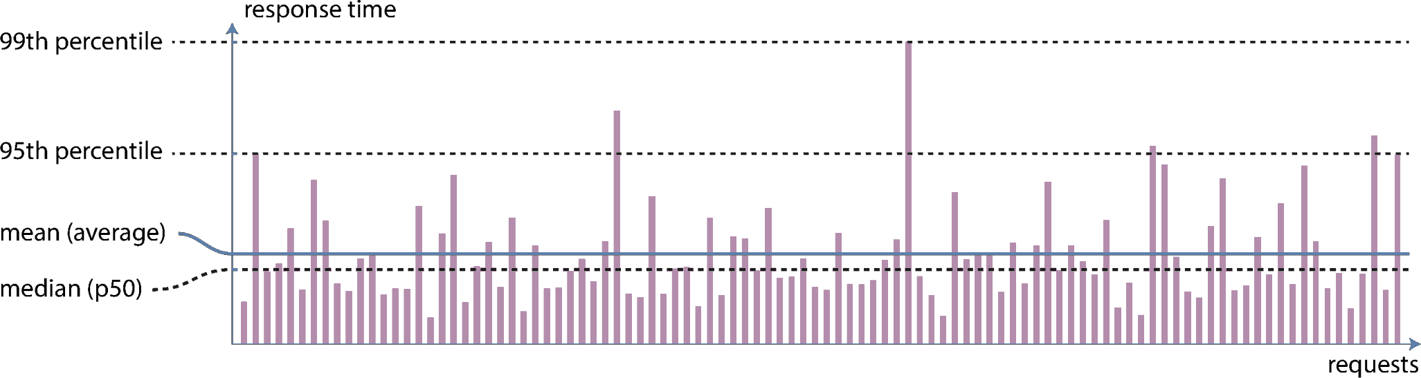
Load and Performance
- Load is characterized by how much work your system is
having to do
- Can vary from system to system, and often times might have several key factors
- Examples: number of requests/queries per second, amount of data to process per second, number of active users
- Changes to load can yield changes in performance
- Often measure through metrics such as records processed per second, or speed of response time
- What is the typical case? – median
- What are the worst cases? – 95%, 99%, or 99.9%
Common Scaling Options
- Scaling Up:
-
- Moving everything over to a more powerful machine
- Often times simpler
- Can get very expensive as the machine needs to get really powerful
- Moving everything over to a more powerful machine
- Scaling Out:
-
- Distributing the load across more machines
- Can be more complicated, but each machine can be cheaper
- Need methods for deciding when more machines need to be added
- Distributing the load across more machines
Maintainability
- Other people who work on the system should be able to work
on it productively.
- Time spent fixing things that broke because you didn’t account for them (and should have) is not productive time
- Time spent jumping back and forth between various systems trying to figure out how they are talking to one another because you over-complicated the system is not productive time
- Time spent having to unpack your system because you did not document it clearly is not productive time
- Non-productive time has very real monetary and resource allocation costs!
Achieving Maintainability
- Operability
- Make it easy for the operations team to keep the system running
smoothly
- Provide transparency in what the system is doing
- Provide excellent documentation of what will happen in specific instances
- Providing good default settings, but allowing manual control when necessary
- Make it easy for the operations team to keep the system running
smoothly
- Simplicity
- Make it easy for others to understand the system, by removing as
much complexity as possible
- Limit complexity that comes just from an implementation
- Use good abstractions, where possible
- Make it easy for others to understand the system, by removing as
much complexity as possible
- Evolvability
- Make it easy for others to make changes to the system in the future
(you’ll never anticipate everything!)
- Use Agile working patterns where possible
- Test-driven development can be useful
- Make it easy for others to make changes to the system in the future
(you’ll never anticipate everything!)
Data Generation
A Plunge into the Data Engineering Lifecycle
- Previously, we showcased the data lifecycle

Generation
- Data can come from a massive variety of sources
- It is up to the data engineer to understand all the different types
of sources and how they might impact future parts of the data lifecycle
- How long does the data persist in the source system?
- At what rate is the data generated?
- How often do errors or formatting issues occur?
- Could the data contain duplicates?
- What schema is used? What happens if it changes?
- How frequently should data be pulled from the source?
- Will reading from the source impact its performance?
Where Could Data Come From?
- As we look toward ingesting data into our data pipeline, we need to
know where it could be coming from
- Files and unstructured data
- APIs
- Application databases
- Analytical databases
- Change Data Capture
- Logs
- Insert-only tables
- Messages and streams
Files
- A universal method of data exchange
- File types each have their quirks and can come in a variety of
structures
- Structured
- Excel, CSV
- Semi-structured
- JSON, XML, CSV
- Unstructured
- TXT
- Structured
APIs
- An application programming interface, or API, is a structure to enable requesting (or modifying) data from another system
- If well crafted, should in theory simply life for data engineers
- In practice, there are can be a wide variety of API formats, and
each tends to be bespoke for the data is works with
- Maintaining many custom API connections can still take considerable time and energy
Application Databases
- Sometimes called transactional databases, these are systems that specialize in online transaction processing (OLTP)
- Focus on supporting and enabling massive amounts of transactions with little latency
- Less suited for analytics, where one query might need to scan or process a vast amount of data
Trippin’ ACID
- Transaction databases will commonly support ACID characteristics
- Atomicity: related transactions all occur at the same time and as a group
- Consistency: reading a value from the database will always return the latest value
- Isolation: if two updates occur at seemingly the same time, the end database state will be consistent with the order they were sent
- Durability: committed data will never be lost, even if power is lost
- Not all systems support all of these, as significant performance boosts can be had from relaxing some of these constraints
Analytical Databases
- Systems constructed to support mainly online analytical processing (OLAP) uses
- Constructed to quickly scan vast amounts of infomation and perform bulk aggregates
- Poorly suited for high amounts of transactions or lookups
Change Data Capture
- Extracts each change event that occurs on a database
- This is akin to tracking changes when you are editing a document: only the change is specified, not the absolute or original values
- Frequently used to replicate information between databases without actually needing to query the database
- Generally handled a bit differently depending on database type
Logs
- Capture information about events happening on a system
- At a minimum, should include:
- Who: what human, computer, or service caused the event?
- What: what actual event occurred?
- When: when did the event transpire?
- Can be encoded in a variety of formats:
- Binary encodings: fast and efficient but less flexible in how they can be used
- Semistructured logs: encoded as text in some serializable format (often JSON)
- Unstructured: essentially plain-text console output. Extracting needed information can be complicated
- Databases frequently store their own write-ahead logs
Messages and Streams
- A message is row data communicated across two or more
systems
- Once the message is received, it is deleted
- Frequently might use a message queue where messages wait until processed (and are then deleted)
- A stream is an append-only log of events
- Can view as a running collection of the latest messages
- Events are ordered by some method (frequently timestamp)
- Let’s you look at trends across many events
Storage
- Every part of the lifecycle depends on some type of storage
- Often, multiple types of storage may be used throughout the cycle
- Key things to keep in mind when evaluating storage options include:
- Can this storage system keep up with the necessary read and write speeds?
- Do you understand the system well enough to know if you are using it non-optimally?
- Can the system scale over time (both in size and performance)?
- Is it pure object storage, or does it need to support complex queries?
- What schema system does the storage solution utilize?
- How hot or cold is the data you need to store?
Beyond Relational
Database Landscape
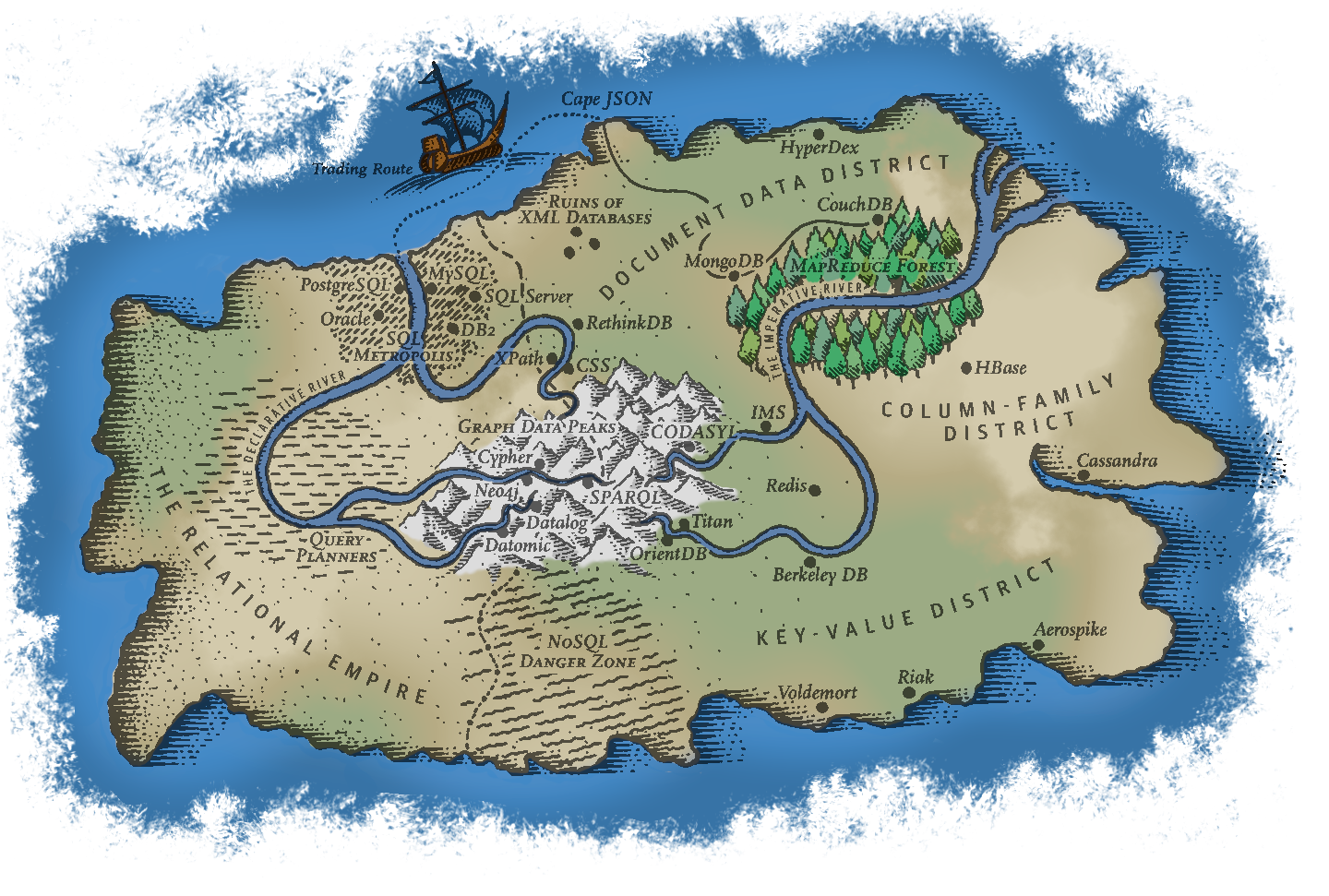
A Choice
- As can be seen from the air, there are a lot of potential database models
- Don’t try to have an in-depth understanding of them all!
- Understand the main groupings so that you can make informed choices
about what might work best in your instance
- All have pros and cons. No “one size fits all” approach is going to work.
- Working out what you need up front will save you lots of time (and effort) in the long run
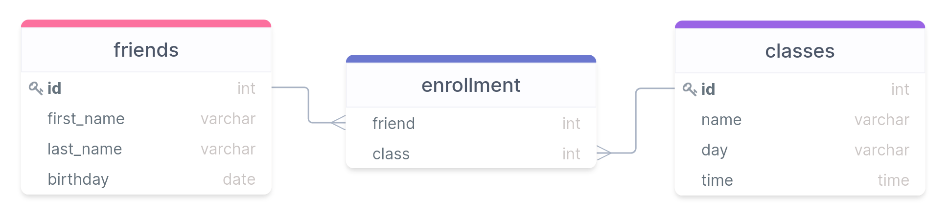
Relational Models
- Principle query language: SQL
- Built on series of tables with matched rows or values linking them (forming the “relationships”)
- Originally built largely for Business Data Processing
- Realized later that it generalized surprisingly well for a much wider set of use cases
- Was widely adopted by the 80’s, and remains the most common and well known data model 40+ years later
The Champion
- Multiple other contenders and technology have arisen, but none have yet displaced SQL and relational models
- SQL does a lot of things very well, but it does have some issues:
- Some datasets have a need for more scalability than relational databases can easily achieve
- Free and open source technologies are all the rage these days, and many flavors of SQL are still largely commercially run products
- Relational schema are restrictive, and some data needs more flexibility
- An object-oriented program impedance mismatch, owing to a disconnect in how each thing about information
- On the plus side, it handles one-to-many and many-to-many
relationships decently well with its relationships, it just means the
information is spread out over potentially many tables
- The power of joins though means this information can be collected together quickly when needed
The Document Model
- Sometimes referred to generally as NoSQL to highlight its differences from relational models
- Best for situations where data exists largely in self-contained documents and outside relationships are fairly rare
- Major examples: XML, JSON, MongoDB
- One-to-many relationships give rise to a tree structure
The Document Model Pros/Cons
- Strength of the document model:
- It handles one-to-many relationships very well
- More closely mimics object-oriented programming, so less impedance mismatch
- Schema are generally quite flexible: not every record has to have the exact same information
- Data is generally stored together or close to related data, so lookups can be fairly efficient
- Weaknesses of the document model
- Struggles more with many-to-many relationships
- Joins are more difficult, and possibly need to be done entirely outside the database in some cases
The Graph Model
- Primarily deals with data with lots of many-to-many relationships
- Relational databases can do this to some extent, but graph models do it really well
- Broken up into:
- Vertices: the information
- Edges: the connections
- Examples: Cypher, SparQL
Our Powers Combined
“It seems that relational and document databases are becoming more similar over time, and that is a good thing: the data models complement each other. If a database is able to handle document-like data and also perform relational queries on it, applications can use the combination of features that best fits their needs. A hybrid of the relational and document models is a good route for databases to take in the future.”
Declarative vs Imperative
- Tells the computer exactly what you want to have happen and in what order
- The way most programming languages work
- Pros:
- Fine grain control
- Highly flexible
- Cons:
- Usually more verbose
- Changes would generally break queries
- Tells the computer what you would like to have occur
- Leaves the details up to the system for how to accomplish that
- Pros:
- More concise and easier to work with
- Abstracts away the complexity, so background work won’t break queries
- Cons
- Need to operate within allowed bounds
- Sometimes less transparency in what is occurring behind the scenes
Break Time
- Get some food and relax!
Data Types
Data Type Fundamentals
- Each column in a table can only have data of a
single type
- Or be missing an entry, designated with a special
NULLentry
- Or be missing an entry, designated with a special
- Assigning the correct data types of columns can
- Improve memory allocations
- Improve performance
- Prevent errors in data entry
- Prevent mistakes in calculations
- Postgres can accept a large number of data types, but today we will focus in depth on the most common: characters, numbers, and dates and times
Characters or Text
- One of the more common things to be stored are characters or sequences of characters
- Postgres has several types you can use to store this sort of
information:
CHAR(|||n|||): A fixed length column of n characters. Always uses this amount of characters, padding with spaces if your stored sequence of characters is shorter.- Omitting the
(|||n|||)is the same asCHAR(1)
- Omitting the
VARCHAR(|||n|||): A variable length column with a maximum of n characters. If your stored sequence is smaller, then no padding is done and the data is stored as is.- Omitting the
(|||n|||)is the same asTEXT
- Omitting the
TEXT★: A variable length column of “unlimited length” (about 1 GB).
- In Postgres (unlike in some other variants) there is not really a difference in performance between all 3 types
★ – Postgres specific, though similar implementations exist in other variants
Character Takeaways
- In general, don’t use
CHARunless what you are storing is always a given length of characters- State abbreviations for instance, or possibly other single character encodings
- Use
VARCHARorTEXTin most situationsVARCHARis more portable, but make sure to choose a max that is well above whatever your longest sequence of characters could be- Can also choose
VARCHARif you want an error to be output if too many characters are entered - If you don’t mind being Postgres specific,
TEXTshould always work
Numbers
- Important to be able to do built-in math calculations on columns
- If the information you want to store is numeric, always use a numeric data type rather than the characters of a number
- A few different options for numbers:
- Integers: whole numbers (positive and negative)
- Fixed-point and Floating-point: fractions of whole numbers (also positive and negative)
- For each there are several data types that you can choose from, largely depending on the size of the numbers you are expecting.
Integers
- Probably the most common form of number you will use in a database
- Can use 3 different data types in SQL to represent an integer
- Differ just in the size of the numbers they can hold
Type Size Range SMALLINT2 bytes ±32,767 INTEGER4 bytes ±2,147,483,648 BIGINT8 bytes ±9,223,372,036,854,775,808 SMALLINTis generally only used if disk space is at a premium- Probably only use
BIGINTif sure thatINTEGERis insufficient
Serial Integers
- If you want a column to be auto-incrementing, you can use the serial
form of the integer types:
SMALLSERIALSERIALBIGSERIAL
- No need to specify that column when adding a row: Postgres will automatically increment and add it
- While each increment will be unique, you may not have perfect even
intervals
- Removed row values are not reused
- If an
INSERTis interrupted because of an error, that unique integer is basically skipped
Your Identity
The
SERIALdatatypes are Postgres specificSince Postgres 10 the SQL core version with
IDENTITYhas been supportedAutomatically fill the column with the incremented number:
INTEGER GENERATED ALWAYS AS IDENTITYAutomatically fill column but allow overwriting:
INTEGER GENERATED BY DEFAULT AS IDENTITY
Fixed-Point Numbers
- Represents a fractional value
- Two methods of writing:
NUMERIC(|||precision|||, |||scale|||)DECIMAL(|||precision|||, |||scale|||)
- precision is a positive integer representing the max total
number of digits comprising the number (on both sides of the decimal
point)
- If provided, needs to be between 1 and 1000
- scale is a positive integer representing the total number of digits to the right of the decimal point
- Will round or pad the decimal digits with 0’s if needed to get the correct number of digits after the decimal
- Will return an error if the input number can’t fit within the precision
Fixed-Point Examples
- Consider the number: 192.837465
- In various fixed-point formats:
NUMERIC(5,2)= 192.84NUMERIC(10,2)= 192.84NUMERIC(15,10)= 192.8374650000NUMERIC(6,3)= 192.837NUMERIC(4,2)= ERROR
- If you don’t include inputs:
NUMERIC(5)= 193- Treats the scale as 0
NUMERIC= 192.837465- Will store up to the maximum precision and scale allowed (131,072 digits before and 16,383 digits after the decimal, lol)
Floating-Point Numbers
- Still represents a fractional value
- Differs from Fixed-Point in that they use exponents to store the information, so the decimal point could “float”
- Two data types that can be used:
REALDOUBLE PRECISION
- They differ just in their precision (and how much storage space they
take)
REALwill show at most 9 significant digits and takes up 4 bytesDOUBLE PRECISIONwill show at most 17 significant digits and takes up 8 bytes
Floating Pitfalls
- Float-point representations are computed using binary math to make them easy to store in the computer
- Some fractional values cannot be perfectly captured with a binary
decimal though
- In the same way that we can’t exactly write 1/3 as a decimal
- Postgres will use the best approximation that it can given the precision, but it is still an approximation!
- Takeaways:
- Do not use floating-point values if you will be doing
sensitive calculations with the numbers!
- i.e. money
- Comparing two float-point values for equality might not work as
expected, due to these tiny approximations
- Better to check if greater or less than, or within a small interval around the desired value
- Do not use floating-point values if you will be doing
sensitive calculations with the numbers!
Dates and Times
- One very nice aspect of all SQL databases is that they can work with
times and dates very easily, assuming the correct data type is used
- This shouldn’t be trivialized! Working with times and dates is often a pain given all the complexities of the Gregorian calendar, time zones, daylight savings time, etc.
- Approximately 4 major time and date data types, summarized in the below table
| Name | Storage Size | Lowest | Highest | Resolution |
|---|---|---|---|---|
DATE |
4 bytes | 4713 BC | 5874897 AD | 1 day |
TIME |
8 bytes | 00:00:00 | 24:00:00 | 1 μs |
TIMESTAMP |
8 bytes | 4713 BC | 294276 AD | 1 μs |
INTERVAL |
16 bytes | -178000000 yrs | -178000000 yrs | 1 μs |
DATES
- Holds information for a single day
- No information about time
- Data needs to be enclosed in single quotes, like text strings
- Postgres can actually correctly parse a ridiculous number of ways of writing the date, but you can never go wrong with the ISO standard of YYYY-MM-DD
- Other acceptable variants include:
| January 18, 2022 | 1/18/2022 | 01/18/22 |
| 2022-Jan-18 | 18-Jan-2022 | Jan-18-22 |
| 20220118 | Jan 18, 22 |
Times
- Holds information about a single time
- No information about date is stored
- A date CAN be included, but it is largely ignored
- Still needs to be enclosed in single quotes
- Has variants that are both with and without timezone
TIMEis technically without timezoneTIME WITH TIME ZONEis, as expected, including a timezone- Postgres has a shorthand notation for this, called
TIMETZ★ - Due to the way timezones are stored and some issues that arise, using this data type is generally discouraged.
- Postgres has a shorthand notation for this, called
More Times
- ISO time formats looks like HH:MM:SS.FFFF, where the hours are on the 24 hour clock
- Other formats are accepted, including
| 16:05:06 | 16:05 | 04:05 PM |
| 04:05:06.123 PM | 04:05:06 AM |
Timezones
- If specifying a timezone, it comes after the time and there are a
few ways to describe it:
- Abbreviation: PST (for Pacific Standard Time)
- Full name: America/Los_Angeles
- This method requires you to enter the date as well, so that it can tell if daylight savings is active or not!
- UTC Offset: -8 (our clocks are currently 8 hours behind GMT)
- If no timezone is specified, but the field requires one, the system timezone is used
- Examples of times with time zones:
- 04:05:06 PM PST
- 2022-01-18 16:05:06 America/Los_Angeles
- 16:05:06-8
Timestamps
- A
TIMESTAMPfield holds basically both a time and a date - The date portion always needs to come first
- The same properties and formats that apply to each individually apply here as well
- Also have the option of with or without a timezone
TIMESTAMPby itself is without a timezone, as per SQL standardsTIMESTAMP WITH TIME ZONEis with a timezone. Shorthand in Postgres isTIMESTAMPTZ★
- Internally, timestamps with a timezone are always stored in UTC, but then when displayed are converted back to the local timezone
- Examples:
- 2022-01-18 14:30:00
- Jan-18-2022 2:30 PM PST
Intervals
- Represents a span of time
- Generally given by first a number and then by a unit
- Possible units: microsecond, millisecond, second, minute, hour, day, week, month, year, decade, century, millennium
- Abbreviations or plurals of the above also work
- Examples:
- 1 day
- 3 century 2 mins
- 45 ms
- 1 mon 87 us
- Intervals can be used in calculations with other date/time data
types
- Can also be used in comparisons if subtracting timestamps
MORE!
- These are just a small sample of some of the most common data types
- Postgres supports many more!
- Booleans
- Geometric types
- Network address types
- JSON types
- A full list can be found here
- We’ll address others as the come up sporadically through the rest of the semester, but you have the core basics now
Conversions
There are plenty of instances where you may need to convert between types
- Sometimes calculations (coming soon!) need a certain data type
- Sometimes the information was just not stored in the most ideal type
Can use the
CASTfunction to convert between data types (where it makes sense)Core syntax is
CAST(|||column name||| AS |||new data type|||)Postgres has a shorthand conversion syntax that uses double colons:
|||column name|||::|||new data type|||Be aware that casting data to a text string with a maximum size smaller than the data will truncate the conversion to get it to fit, not give an error.
Table Input/Output
SQL I/O
INSERT INTOis great for small tables or adding a few rows, not so great for bulk populating of a table- Frequently, data is stored in delimited text files for flexibility and portability
- Postgres can import data from or write data to these sorts
of delimited text files using its
COPYcommand- This command is Postgres specific, though other SQL variants have their similar methods
- Postgres needs to have permission to access the file or folder in
order to import or export!
- If having issues:
- On Windows: The
C:\Users\Publicshould be universally accessible - On Mac:
/Users/Sharedfolder should be universally accessible, or you could use/tmp(but that gets purged each time you reboot)
- On Windows: The
- If having issues:
Delimited Files
- A delimited text file simply uses a special character, called the delimiter, to indicate where column breaks should be
- Otherwise, each line contains the information for a single row
- Most common delimiter is the comma, and hence the term CSV or
“Comma-Separated Values”
- Basically any character can be used as a delimiter though, so you might need to adjust sometimes
- If the delimiter naturally appears in an entry, and isn’t indicating
a column break, then that entry needs to be surrounded with a text
qualifier
- The most common text qualifier is a pair of double quotes, but it could be other symbols
- Often times, the first row of the file is a delimited description of
each column name or what it represents
- Not always present, in which case you (hopefully) have other documentation to consult to understand the column meanings
An Office-ial CSV
id,first_name,last_name,birthday
1,Michael,Scott,"Mar 15, 1964"
2,Dwight,Schrute,"Jan 20, 1970"
3,Pam,Beesly,"Mar 25, 1979"
4,Jim,Halpert,"Oct 1, 1978"
5,Kelly,Kapoor,"Feb 5, 1980"- Note:
- The birthday column entries are quoted owing to the comma within them
- No spaces show up anywhere except within quoted blocks
- The first line contains a header, which is useful for understanding but contains no actual data
- Make sure you have no empty line at the end!
Importing Data
The
COPYcommand will copy information into an existing table, it won’t create the table- Thus you are still responsible for creating the table (and
associated data types for each column) before
COPYwill be useful- Yes, this can still be painful for huge tables. There are some scripts that can help with it or do some automated checking, but they tend to be far from perfect.
- Thus you are still responsible for creating the table (and
associated data types for each column) before
Syntax of the
COPYstatement:COPY |||table name||| FROM |||'full path to filename'||| WITH ( |||import options||| );
Importing Details
- The full text filename needs to be the entire path that points to
your file
- On Windows, that would start with
C:\ - On MacOS, that would start with
/
- On Windows, that would start with
- You have a basic selection of import options:
FORMAT CSVsets the delimiter to a comma and the default text qualifier to double quotesHEADERspecifies that there is a header, and so the first row of the file should be skippedDELIMITER 'x'setsxto be the delimiter instead of the default comma (or tab)QUOTE 'x'setsxto be the new text qualifier, instead of double quotes
- If you run the
COPYcommand multiple times, it will just keep adding the CSV contents to the end of the current table
Subset Imports
Sometimes an CSV might not have all the data you want in your SQL table
You can import all the information from the CSV into only a subset of the SQL table columns
- As far as I know, you can’t easily go the other direction, importing only a portion of the CSV columns
Just requires that you specify the target SQL columns after specifying the table
COPY |||table name||| (|||col₁|||, |||col₂|||, |||col₃|||)
FROM |||full path to filename|||
WITH (FORMAT CSV, HEADER);
Importing only certain rows
Starting with Postgres 12, the option was added to use a
WHEREkeyword to only copy rows that met a certain condition to the tableThe
WHEREcomes after theWITHstatement:COPY |||table name||| (|||col₁|||, |||col₂|||) FROM |||full path to filename||| WITH (FORMAT CSV) WHERE |||col₂||| = 'Baboon'
Exporting Data
Exporting data takes information from your SQL table and allows you to store it in a text file
- Note that this process isn’t lossless, as the data types of each column are not stored, just the contents and (possibly) column names
Syntax-wise, it is almost exactly like copying into a SQL table, except using
TOinstead ofFROMCOPY |||table name||| TO |||full path to filename||| WITH ( |||import options||| );This exports all columns from the specified table to the filename with the desired format
Exporting Subsets
- In many instances, you may not want all the columns to be exported. In that case, you have a few options:
- Exporting only particular columns:
- Just specify the desired columns after the table name
COPY |||table name||| (|||col₁|||, |||col₂|||, |||col₃|||) TO |||full path to filename||| WITH ( |||import options||| ); - Export just the output of a query:
- Embed the query instead of a table name
COPY (
  SELECT |||col₁|||, |||col₂||| FROM |||table name|||
  ORDER BY |||col₂|||
  )
TO |||full path to filename|||
WITH ( |||import_options||| );