---
title: "The Source of Types and Commerce"
author: Jed Rembold
date: January 22, 2025
slideNumber: true
theme: nord_light
highlightjs-theme: nord
width: 1920
height: 1080
transition: fade
---
## Announcements
- Did the first HW get submitted ok?
- If you had any issues, let's get them figured out before you leave tonight
- My apologies about the Canvas mistake
- Homework 2 is posted! On both the website and Canvas!
- For next week:
- DeBarros: Ch 6
# System Objectives
## The Primary Objective(s)
There are three main concerns when building any data system:
Reliability:
: The system works and is not prone to breakage
Scalability:
: The system can grow as needs or data grows
Maintainability:
: Future work on the system can be done productively
## Secondary Objective
- There are other high-level issues to consider as well
- How do you ensure that the data remains correct and complete?
- How do you handle increased size or data load?
- How should your database interface with users?
- How will you handle errors or problems and the resulting downtime?
## External Factors
- Oftentimes "outside" factors can also influence how your system can be build or managed
- The skill and experience of developers and users
- Any legacy system dependencies
- Time-scale for delivery
- Your organization's tolerance for risk
- Regulatory climate
# Reliability
## Reliability
- **The system should continue to work correctly, even when things go wrong.**
- The application should perform as the user expects
- The application has a reasonable tolerance for errors or unexpected use
- The application achieves the goals of the use case(s)
- The application prevents abuse or unauthorized access
## System Resilience
- A _fault_ is anything that could go wrong in the use of a data system
- Don't necessarily have to break the entire system (system failure)
- A system that can tolerate faults without entirely breaking is said to be _resilient_
- Faults are going to happen! The goal is to gracefully handle them and prevent system failure.
- You can not fully plan/mitigate every potential fault
- At some point, you have to accept that the odds of some faults occurring are not worth the expense it would take to mitigate against them.
## Fault Types!
::::::{.cols style='align-items: center'}
::::{.col style='font-size:.9em'}
Hardware faults:
: - Not if, but **when** hardware will die!
Software faults:
: - Probably less likely, but potentially more devastating, as they tend to cascade.
Human faults:
: - Potentially the most common source
- Can be managed through careful planning and clear communication
::::
::::col
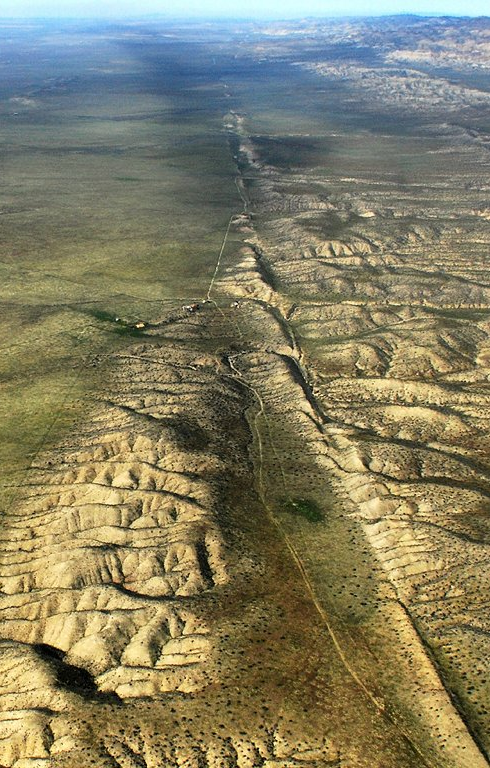{width=60%}
::::
::::::
# Scalability
## Scalability
::::::{.cols style='align-items:center'}
::::col
{width=100%}
::::
::::{.col style='font-size:.9em'}
- As the demands on the data system grow, there should be reasonable options available for handling the increased demand.
- Understanding _exactly_ how a system's demands might grow is usually impossible, but the idea is to have contingencies in place and routes where growth COULD happen.
- "If we grow in this way, what options would we have?"
- Requires being able to quantify when the system needs to grow!
::::
::::::
## Load and Performance
:::{style='font-size=.9em'}
- _Load_ is characterized by how much work your system is having to do
- Can vary from system to system, and often times might have several key factors
- Examples: number of requests/queries per second, amount of data to process per second, number of active users
- Changes to load can yield changes in _performance_
- Often measure through metrics such as records processed per second, or speed of response time
- What is the typical case? -- _median_
- What are the worst cases? -- _95%, 99%, or 99.9%_
:::
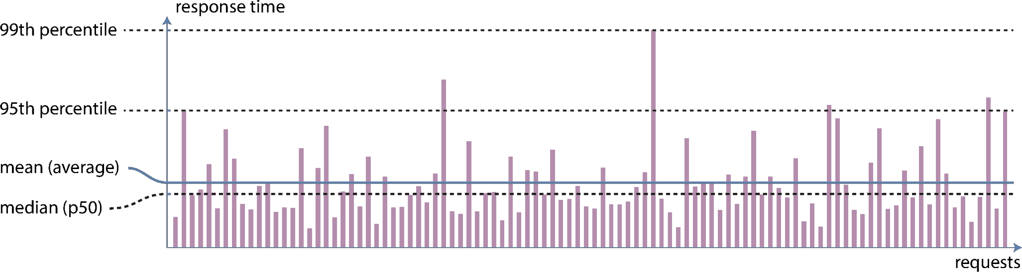{width=50%}
## Common Scaling Options
Scaling Up:
: - Moving everything over to a more powerful machine
- Often times simpler
- Can get very expensive as the machine needs to get really powerful
Scaling Out:
: - Distributing the load across more machines
- Can be more complicated, but each machine can be cheaper
- Need methods for deciding when more machines need to be added
# Maintainability
## Maintainability
- Other people who work on the system **should be able to work on it productively.**
- Time spent fixing things that broke because you didn't account for them (and should have) is not productive time
- Time spent jumping back and forth between various systems trying to figure out how they are talking to one another because you over-complicated the system is not productive time
- Time spent having to unpack your system because you did not document it clearly is not productive time
- Non-productive time has very real monetary and resource allocation costs!
## Achieving Maintainability
:::{style='font-size:.8em'}
- _Operability_
- Make it easy for the operations team to keep the system running smoothly
- Provide transparency in what the system is doing
- Provide excellent documentation of what will happen in specific instances
- Providing good default settings, but allowing manual control when necessary
- _Simplicity_
- Make it easy for others to understand the system, by removing as much complexity as possible
- Limit complexity that comes just from an implementation
- Use good abstractions, where possible
- _Evolvability_
- Make it easy for others to make changes to the system in the future (you'll never anticipate everything!)
- Use _Agile_ working patterns where possible
- Test-driven development can be useful
:::
# Data Generation
## A Plunge into the Data Engineering Lifecycle
- Previously, we showcased the data lifecycle
\begin{tikzpicture}[box/.style={draw=black, thick, rounded corners, font=\sf}]%%width=100%
\node[box, minimum size=1cm, fill=Frost1](gen) at (0,0) {Generation};
\node[box, minimum size=1cm, fill=Frost2, anchor=west, outer sep = 3pt](ing) at ($(gen.east)+(0.75,0.4)$) {Ingestion};
\node[box, minimum size=1cm, fill=Frost3, anchor=west, outer sep = 3pt](trans) at (ing.east) {Transformation};
\node[box, minimum size=1cm, fill=Frost4, anchor=west, outer sep = 3pt](serv) at (trans.east) {Serving};
\path let \p1 = (ing.south west), \p2 = (serv.south east), \n1 = {\x2-\x1-6pt} in
node[box, minimum width=\n1, fill=Purple, anchor=north west, outer sep = 3pt](stor) at (ing.south west) {Storage};
\node[box, line width=3pt, fit=(ing)(trans)(serv)(stor)](lc) {};
\draw[ultra thick, -stealth] (gen.east) -- ($(lc.north west)!(gen.east)!(lc.south west)$) coordinate (gend);
\draw[ultra thick, -stealth] (lc.east) -- +(0.5,0) node[box, minimum width=3cm, fill=Green, anchor=west] {Analytics};
\draw[ultra thick, -stealth] (lc.north east) ++ (0,-.2) -- +(0.5,0) node[box, minimum width=3cm, fill=Green, anchor=west] {Machine Learning};
\draw[ultra thick, -stealth] (lc.south east) ++ (0,0.2) -- +(0.5,0) node[box, minimum width=3cm, fill=Green, anchor=west] {Reverse ETL};
\end{tikzpicture}
## Generation
- Data can come from a **massive** variety of sources
- It is up to the data engineer to understand all the different types of sources and how they might impact future parts of the data lifecycle
- How long does the data persist in the source system?
- At what rate is the data generated?
- How often do errors or formatting issues occur?
- Could the data contain duplicates?
- What schema is used? What happens if it changes?
- How frequently should data be pulled from the source?
- Will reading from the source impact its performance?
## Where Could Data Come From?
- As we look toward ingesting data into our data pipeline, we need to know where it could be coming from
- Files and unstructured data
- APIs
- Application databases
- Analytical databases
- Change Data Capture
- Logs
- Insert-only tables
- Messages and streams
## Files
- A universal method of data exchange
- File types each have their quirks and can come in a variety of structures
- Structured
- Excel, CSV
- Semi-structured
- JSON, XML, CSV
- Unstructured
- TXT
## APIs
- An _application programming interface_, or API, is a structure to enable requesting (or modifying) data from another system
- If well crafted, should in theory simply life for data engineers
- In practice, there are can be a wide variety of API formats, and each tends to be bespoke for the data is works with
- Maintaining many custom API connections can still take considerable time and energy
## Application Databases
- Sometimes called _transactional databases_, these are systems that specialize in _online transaction processing_ (OLTP)
- Focus on supporting and enabling massive amounts of transactions with little latency
- Less suited for analytics, where one query might need to scan or process a vast amount of data
## Trippin' ACID
- Transaction databases will commonly support ACID characteristics
- _Atomicity_: related transactions all occur at the same time and as a group
- _Consistency_: reading a value from the database will always return the latest value
- _Isolation_: if two updates occur at seemingly the same time, the end database state will be consistent with the order they were sent
- _Durability_: committed data will never be lost, even if power is lost
- Not all systems support all of these, as significant performance boosts can be had from relaxing some of these constraints
## Analytical Databases
- Systems constructed to support mainly _online analytical processing_ (OLAP) uses
- Constructed to quickly scan vast amounts of infomation and perform bulk aggregates
- Poorly suited for high amounts of transactions or lookups
## Change Data Capture
- Extracts each _change_ event that occurs on a database
- This is akin to tracking changes when you are editing a document: only the change is specified, not the absolute or original values
- Frequently used to replicate information between databases without actually needing to query the database
- Generally handled a bit differently depending on database type
## Logs
- Capture information about events happening on a system
- At a minimum, should include:
- _Who_: what human, computer, or service caused the event?
- _What_: what actual event occurred?
- _When_: when did the event transpire?
- Can be encoded in a variety of formats:
- Binary encodings: fast and efficient but less flexible in how they can be used
- Semistructured logs: encoded as text in some serializable format (often JSON)
- Unstructured: essentially plain-text console output. Extracting needed information can be complicated
- Databases frequently store their own _write-ahead logs_
## Messages and Streams
- A _message_ is row data communicated across two or more systems
- Once the message is received, it is deleted
- Frequently might use a message queue where messages wait until processed (and are then deleted)
- A stream is an append-only log of events
- Can view as a running collection of the latest messages
- Events are ordered by some method (frequently timestamp)
- Let's you look at trends across many events
## Storage
- Every part of the lifecycle depends on some type of storage
- Often, multiple types of storage may be used throughout the cycle
- Key things to keep in mind when evaluating storage options include:
- Can this storage system keep up with the necessary read and write speeds?
- Do you understand the system well enough to know if you are using it non-optimally?
- Can the system scale over time (both in size and performance)?
- Is it pure object storage, or does it need to support complex queries?
- What schema system does the storage solution utilize?
- How hot or cold is the data you need to store?
# Beyond Relational
## Database Landscape
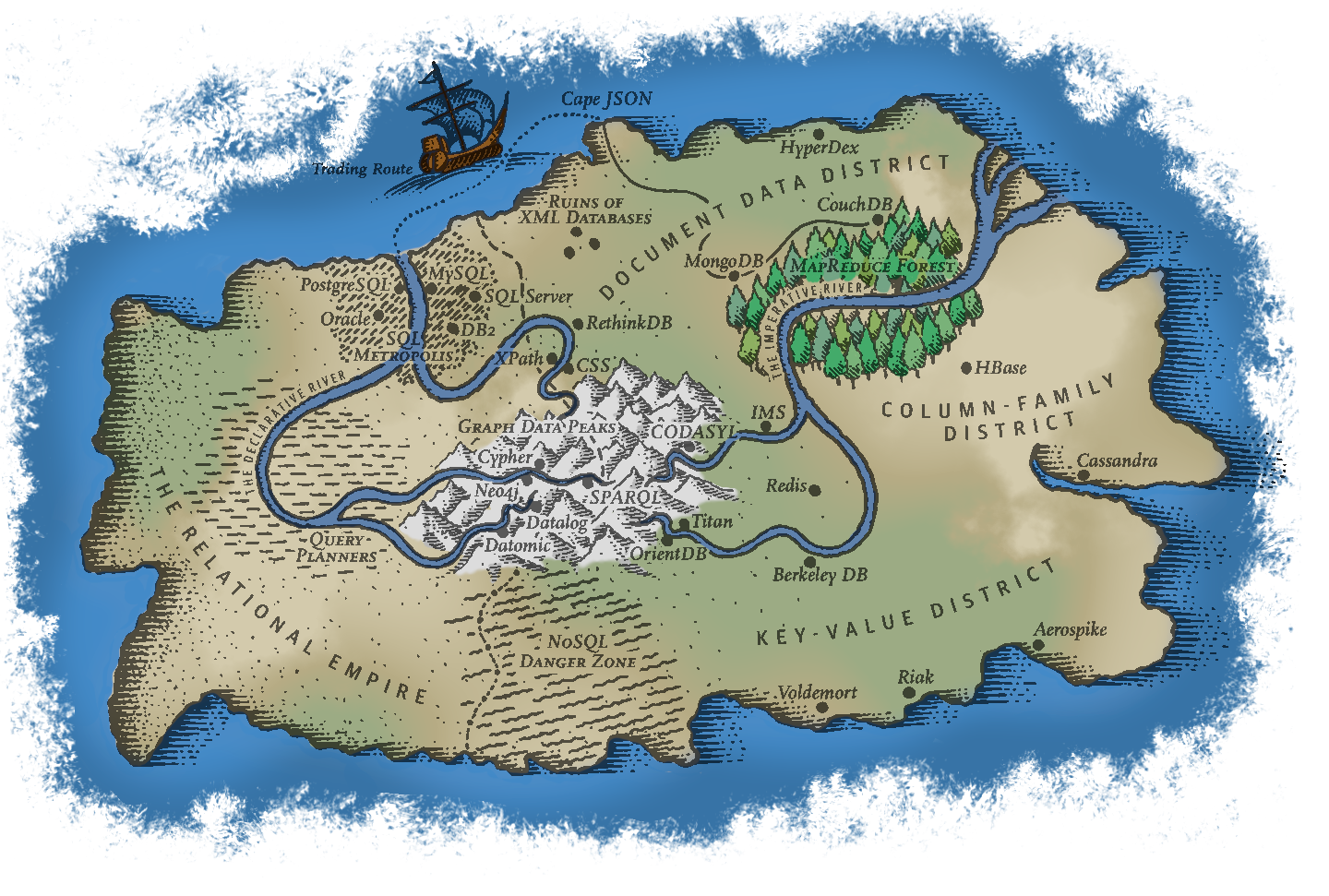{width=75%}
## A Choice
- As can be seen from the air, there are a _lot_ of potential database models
- Don't try to have an in-depth understanding of them all!
- Understand the main groupings so that you can make informed choices about what might work best in your instance
- All have pros and cons. No "one size fits all" approach is going to work.
- Working out what you need up front will save you lots of time (and effort) in the long run
{width=50%}
## Relational Models
- Principle query language: SQL
- Built on series of tables with matched rows or values linking them (forming the "relationships")
- Originally built largely for Business Data Processing
- Realized later that it generalized surprisingly well for a much wider set of use cases
- Was widely adopted by the 80's, and remains the most common and well known data model 40+ years later
{width=60%}
## The Champion
:::{style='font-size:.9em'}
- Multiple other contenders and technology have arisen, but none have yet displaced SQL and relational models
- SQL does a lot of things very well, but it does have some issues:
- Some datasets have a need for more scalability than relational databases can easily achieve
- Free and open source technologies are all the rage these days, and many flavors of SQL are still largely commercially run products
- Relational schema are restrictive, and some data needs more flexibility
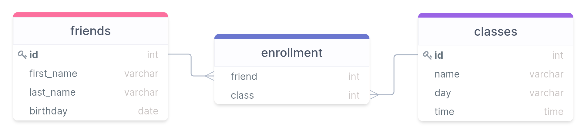
- An object-oriented program _impedance mismatch_, owing to a disconnect in how each thing about information
- On the plus side, it handles one-to-many and many-to-many relationships decently well with its relationships, it just means the information is spread out over potentially many tables
- The power of joins though means this information can be collected together quickly when needed
:::
## The Document Model
::::::cols
::::col
- Sometimes referred to generally as NoSQL to highlight its differences from relational models
- Best for situations where data exists largely in self-contained documents and outside relationships are fairly rare
- Major examples: XML, JSON, MongoDB
- One-to-many relationships give rise to a tree structure
::::
::::col

::::
::::::
## The Document Model Pros/Cons
- Strength of the document model:
- It handles one-to-many relationships very well
- More closely mimics object-oriented programming, so less impedance mismatch
- Schema are generally quite flexible: not every record has to have the exact same information
- Data is generally stored together or close to related data, so lookups can be fairly efficient
- Weaknesses of the document model
- Struggles more with many-to-many relationships
- Joins are more difficult, and possibly need to be done entirely outside the database in some cases
## The Graph Model
::::::cols
::::col
- Primarily deals with data with lots of many-to-many relationships
- Relational databases can do this to some extent, but graph models do it really well
- Broken up into:
- Vertices: the information
- Edges: the connections
- Examples: Cypher, SparQL
::::
::::col

::::
::::::
## Our Powers Combined
> “It seems that relational and document databases are becoming more similar over time, and that is a good thing: the data models complement each other. If a database is able to handle document-like data and also perform relational queries on it, applications can use the combination of features that best fits their needs. A hybrid of the relational and document models is a good route for databases to take in the future.”
## Declarative vs Imperative
::::::cols
::::col
:::{.block name=Imperative}
- Tells the computer exactly what you want to have happen and in what order
- The way most programming languages work
- Pros:
- Fine grain control
- Highly flexible
- Cons:
- Usually more verbose
- Changes would generally break queries
:::
::::
::::col
:::{.block name=Declarative}
- Tells the computer what you would like to have occur
- Leaves the details up to the system for how to accomplish that
- Pros:
- More concise and easier to work with
- Abstracts away the complexity, so background work won't break queries
- Cons
- Need to operate within allowed bounds
- Sometimes less transparency in what is occurring behind the scenes
:::
::::
::::::
## Break Time
- Get some food and relax!
# Data Types
## Data Type Fundamentals
- Each column in a table can only have data of a **single** type
- Or be missing an entry, designated with a special `NULL` entry
- Assigning the correct data types of columns can
- Improve memory allocations
- Improve performance
- Prevent errors in data entry
- Prevent mistakes in calculations
- Postgres can accept a _large_ number of data types, but today we will focus in depth on the most common: characters, numbers, and dates and times
## Characters or Text{data-notes="Example after this"}
:::{style='font-size:.9em'}
- One of the more common things to be stored are characters or sequences of characters
- Postgres has several types you can use to store this sort of information:
- `CHAR(|||n|||)`: A fixed length column of _n_ characters. **Always** uses this amount of characters, padding with spaces if your stored sequence of characters is shorter.
- Omitting the `(|||n|||)` is the same as `CHAR(1)`{.pgsql}
- `VARCHAR(|||n|||)`: A variable length column with a **maximum** of _n_ characters. If your stored sequence is smaller, then no padding is done and the data is stored as is.
- Omitting the `(|||n|||)` is the same as `TEXT`{.pgsql}
- `TEXT`[★]{.orange}: A variable length column of "unlimited length" (about 1 GB).
- In Postgres (unlike in some other variants) there is not really a difference in performance between all 3 types
:::
:::{style='font-size:.8em'}
[★]{.orange} -- Postgres specific, though similar implementations exist in other variants
:::
## Character Takeaways
- In general, don't use `CHAR` unless what you are storing is _always_ a given length of characters
- State abbreviations for instance, or possibly other single character encodings
- Use `VARCHAR` or `TEXT` in most situations
- `VARCHAR` is more portable, but make sure to choose a max that is well above whatever your longest sequence of characters could be
- Can also choose `VARCHAR` if you _want_ an error to be output if too many characters are entered
- If you don't mind being Postgres specific, `TEXT` should always work
## Numbers
- Important to be able to do built-in math calculations on columns
- If the information you want to store is numeric, always use a numeric data type rather than the characters of a number
- A few different options for numbers:
- _Integers_: whole numbers (positive and negative)
- _Fixed-point_ and _Floating-point_: fractions of whole numbers (also positive and negative)
- For each there are several data types that you can choose from, largely depending on the size of the numbers you are expecting.
## Integers
- Probably the most common form of number you will use in a database
- Can use 3 different data types in SQL to represent an integer
- Differ just in the size of the numbers they can hold
Type | Size | Range
--- | --- | ---
`SMALLINT` | 2 bytes | ±32,767
`INTEGER` | 4 bytes | ±2,147,483,648
`BIGINT` | 8 bytes | ±9,223,372,036,854,775,808
- `SMALLINT` is generally only used if disk space is at a premium
- Probably only use `BIGINT` if sure that `INTEGER` is insufficient
## Serial Integers
- If you want a column to be auto-incrementing, you can use the serial form of the integer types:
- `SMALLSERIAL`
- `SERIAL`
- `BIGSERIAL`
- No need to specify that column when adding a row: Postgres will automatically increment and add it
- While each increment will be unique, you may not have perfect even intervals
- Removed row values are not reused
- If an `INSERT` is interrupted because of an error, that unique integer is basically skipped
## Your Identity
- The `SERIAL` datatypes are Postgres specific
- Since Postgres 10 the SQL core version with `IDENTITY` has been supported
- Automatically fill the column with the incremented number:
```pgsql
INTEGER GENERATED ALWAYS AS IDENTITY
```
- Automatically fill column but allow overwriting:
```pgsql
INTEGER GENERATED BY DEFAULT AS IDENTITY
```
## Fixed-Point Numbers
:::{style='font-size:.9em'}
- Represents a fractional value
- Two methods of writing:
- `NUMERIC(|||precision|||, |||scale|||)`
- `DECIMAL(|||precision|||, |||scale|||)`
- _precision_ is a positive integer representing the max total number of digits comprising the number (on both sides of the decimal point)
- If provided, needs to be between 1 and 1000
- _scale_ is a positive integer representing the total number of digits to the right of the decimal point
- Will round or pad the decimal digits with 0's if needed to get the correct number of digits after the decimal
- Will return an error if the input number can't fit within the precision
:::
## Fixed-Point Examples
- Consider the number: 192.837465
- In various fixed-point formats:
- `NUMERIC(5,2)` = 192.84
- `NUMERIC(10,2)` = 192.84
- `NUMERIC(15,10)` = 192.8374650000
- `NUMERIC(6,3)` = 192.837
- `NUMERIC(4,2)` = **ERROR**
- If you don't include inputs:
- `NUMERIC(5)` = 193
- Treats the scale as 0
- `NUMERIC` = 192.837465
- Will store up to the maximum precision and scale allowed (131,072 digits before and 16,383 digits after the decimal, lol)
## Floating-Point Numbers
- Still represents a fractional value
- Differs from Fixed-Point in that they use exponents to store the information, so the decimal point could "float"
- Two data types that can be used:
- `REAL`
- `DOUBLE PRECISION`
- They differ just in their precision (and how much storage space they take)
- `REAL` will show at most 9 significant digits and takes up 4 bytes
- `DOUBLE PRECISION` will show at most 17 significant digits and takes up 8 bytes
## Floating Pitfalls
:::{style='font-size:.9em'}
- Float-point representations are computed using binary math to make them easy to store in the computer
- Some fractional values cannot be perfectly captured with a binary decimal though
- In the same way that we can't _exactly_ write 1/3 as a decimal
- Postgres will use the best approximation that it can given the precision, but it is still an approximation!
- Takeaways:
- **Do not use floating-point values if you will be doing sensitive calculations with the numbers!**
- i.e. money
- Comparing two float-point values for equality might not work as expected, due to these tiny approximations
- Better to check if greater or less than, or within a small interval around the desired value
:::
## Dates and Times
- One very nice aspect of all SQL databases is that they can work with times and dates very easily, assuming the correct data type is used
- This shouldn't be trivialized! Working with times and dates is often a **pain** given all the complexities of the Gregorian calendar, time zones, daylight savings time, etc.
- Approximately 4 major time and date data types, summarized in the below table
Name | Storage Size | Lowest | Highest | Resolution
--- |---|---|---|---
`DATE` | 4 bytes | 4713 BC | 5874897 AD | 1 day
`TIME` | 8 bytes | 00:00:00 | 24:00:00 | 1 μs
`TIMESTAMP` | 8 bytes | 4713 BC | 294276 AD | 1 μs
`INTERVAL` | 16 bytes | -178000000 yrs | -178000000 yrs | 1 μs
## DATES
- Holds information for a single day
- No information about time
- Data needs to be enclosed in single quotes, like text strings
- Postgres can actually correctly parse a ridiculous number of ways of writing the date, but you can never go wrong with the ISO standard of YYYY-MM-DD
- Other acceptable variants include:
----------------- ------------- ---------------
January 18, 2022 1/18/2022 01/18/22
2022-Jan-18 18-Jan-2022 Jan-18-22
20220118 Jan 18, 22
----------------- ------------- ---------------
## Times
- Holds information about a single time
- No information about date is stored
- A date CAN be included, but it is largely ignored
- Still needs to be enclosed in single quotes
- Has variants that are both with and without timezone
- `TIME` is technically without timezone
- `TIME WITH TIME ZONE` is, as expected, including a timezone
- Postgres has a shorthand notation for this, called `TIMETZ`[★]{.orange}
- Due to the way timezones are stored and some issues that arise, using this data type is generally discouraged.
## More Times
- ISO time formats looks like HH:MM:SS.FFFF, where the hours are on the **24 hour clock**
- Other formats are accepted, including
----------------- ------------- ---------------
16:05:06 16:05 04:05 PM
04:05:06.123 PM 04:05:06 AM
----------------- ------------- ---------------
## Timezones
:::{style='font-size:.9em'}
- If specifying a timezone, it comes after the time and there are a few ways to describe it:
- Abbreviation: PST (for Pacific Standard Time)
- Full name: America/Los_Angeles
- This method requires you to enter the date as well, so that it can tell if daylight savings is active or not!
- UTC Offset: -8 (our clocks are currently 8 hours behind GMT)
- If no timezone is specified, but the field requires one, the system timezone is used
- Examples of times with time zones:
- 04:05:06 PM PST
- 2022-01-18 16:05:06 America/Los_Angeles
- 16:05:06-8
:::
## Timestamps
:::{style='font-size:.9em'}
- A `TIMESTAMP` field holds basically both a time and a date
- The date portion always needs to come first
- The same properties and formats that apply to each individually apply here as well
- Also have the option of with or without a timezone
- `TIMESTAMP` by itself is without a timezone, as per SQL standards
- `TIMESTAMP WITH TIME ZONE` is with a timezone. Shorthand in Postgres is `TIMESTAMPTZ`[★]{.orange}
- Internally, timestamps with a timezone are always _stored_ in UTC, but then when displayed are converted back to the local timezone
- Examples:
- 2022-01-18 14:30:00
- Jan-18-2022 2:30 PM PST
:::
## Intervals
:::{style='font-size:.9em'}
- Represents a span of time
- Generally given by first a number and then by a unit
- Possible units: microsecond, millisecond, second, minute, hour, day, week, month, year, decade, century, millennium
- Abbreviations or plurals of the above also work
- Examples:
- 1 day
- 3 century 2 mins
- 45 ms
- 1 mon 87 us
- Intervals can be used in calculations with other date/time data types
- Can also be used in comparisons if subtracting timestamps
:::
## MORE!
- These are just a small sample of some of the most common data types
- Postgres supports _many_ more!
- Booleans
- Geometric types
- Network address types
- JSON types
- A full list can be found [here](https://www.postgresql.org/docs/14/datatype.html)
- We'll address others as the come up sporadically through the rest of the semester, but you have the core basics now
## Conversions
:::{style='font-size:.9em'}
- There are plenty of instances where you may need to convert between types
- Sometimes calculations (coming soon!) need a certain data type
- Sometimes the information was just not stored in the most ideal type
- Can use the `CAST` function to convert between data types (where it makes sense)
- Core syntax is
```pgsql
CAST(|||column name||| AS |||new data type|||)
```
- Postgres has a shorthand conversion syntax that uses double colons:
```pgsql
|||column name|||::|||new data type|||
```
- Be aware that casting data to a text string with a maximum size smaller than the data will _truncate_ the conversion to get it to fit, _not_ give an error.
:::
# Table Input/Output
## SQL I/O
:::{style='font-size:.9em'}
- `INSERT INTO` is great for small tables or adding a few rows, not so great for bulk populating of a table
- Frequently, data is stored in delimited text files for flexibility and portability
- Postgres can import data from _or_ write data to these sorts of delimited text files using its `COPY` command
- This command is Postgres specific, though other SQL variants have their similar methods
- Postgres needs to have permission to access the file or folder in order to import or export!
- If having issues:
- On Windows: The `C:\Users\Public`{.text} should be universally accessible
- On Mac: `/Users/Shared` folder should be universally accessible, or you could use `/tmp` (but that gets purged each time you reboot)
:::
## Delimited Files
:::{style='font-size:.9em'}
- A delimited text file simply uses a special character, called the _delimiter_, to indicate where column breaks should be
- Otherwise, each line contains the information for a single row
- Most common delimiter is the comma, and hence the term CSV or "Comma-Separated Values"
- Basically any character can be used as a delimiter though, so you might need to adjust sometimes
- If the delimiter naturally appears in an entry, and isn't indicating a column break, then that entry needs to be surrounded with a _text qualifier_
- The most common text qualifier is a pair of double quotes, but it could be other symbols
- Often times, the first row of the file is a delimited description of each column name or what it represents
- Not always present, in which case you (hopefully) have other documentation to consult to understand the column meanings
:::
## An Office-ial CSV
```text
id,first_name,last_name,birthday
1,Michael,Scott,"Mar 15, 1964"
2,Dwight,Schrute,"Jan 20, 1970"
3,Pam,Beesly,"Mar 25, 1979"
4,Jim,Halpert,"Oct 1, 1978"
5,Kelly,Kapoor,"Feb 5, 1980"
```
- Note:
- The birthday column entries are quoted owing to the comma within them
- No spaces show up anywhere except within quoted blocks
- The first line contains a header, which is useful for understanding but contains no actual data
- Make sure you have no empty line at the end!
## Importing Data
- The `COPY` command will copy information into an _existing_ table, it won't create the table
- Thus you are still responsible for creating the table (and associated data types for each column) before `COPY` will be useful
- Yes, this can still be painful for huge tables. There are some scripts that can help with it or do some automated checking, but they tend to be far from perfect.
- Syntax of the `COPY` statement:
```pgsql
COPY |||table name|||
FROM |||'full path to filename'|||
WITH ( |||import options||| );
```
## Importing Details
:::{style='font-size:.9em'}
- The full text filename needs to be the entire path that points to your file
- On Windows, that would start with `C:\`
- On MacOS, that would start with `/`
- You have a basic selection of import options:
- `FORMAT CSV` sets the delimiter to a comma and the default text qualifier to double quotes
- `HEADER` specifies that there is a header, and so the first row of the file should be skipped
- `DELIMITER 'x'` sets `x` to be the delimiter instead of the default comma (or tab)
- `QUOTE 'x'` sets `x` to be the new text qualifier, instead of double quotes
- If you run the `COPY` command multiple times, it will just keep adding the CSV contents to the end of the current table
:::
## Subset Imports
- Sometimes an CSV might not have _all_ the data you want in your SQL table
- You can import all the information from the CSV into only a subset of the SQL table columns
- As far as I know, you can't easily go the other direction, importing only a portion of the CSV columns
- Just requires that you specify the target SQL columns after specifying the table
```pgsql
COPY |||table name||| (|||col₁|||, |||col₂|||, |||col₃|||)
FROM |||full path to filename|||
WITH (FORMAT CSV, HEADER);
```
## Importing only certain rows
- Starting with Postgres 12, the option was added to use a `WHERE` keyword to only copy rows that met a certain condition to the table
- The `WHERE` comes _after_ the `WITH` statement:
```pgsql
COPY |||table name||| (|||col₁|||, |||col₂|||)
FROM |||full path to filename|||
WITH (FORMAT CSV)
WHERE |||col₂||| = 'Baboon'
```
## Exporting Data
- Exporting data takes information from your SQL table and allows you to store it in a text file
- Note that this process isn't lossless, as the data types of each column are not stored, just the contents and (possibly) column names
- Syntax-wise, it is almost exactly like copying into a SQL table, except using `TO` instead of `FROM`
```pgsql
COPY |||table name|||
TO |||full path to filename|||
WITH ( |||import options||| );
```
- This exports **all** columns from the specified table to the filename with the desired format
## Exporting Subsets
:::{style="font-size:.8em"}
- In many instances, you may not want **all** the columns to be exported. In that case, you have a few options:
- Exporting only particular columns:
- Just specify the desired columns after the table name
```{.pgsql style="font-size:1em;"}
COPY |||table name||| (|||col₁|||, |||col₂|||, |||col₃|||)
TO |||full path to filename|||
WITH ( |||import options||| );
```
- Export just the output of a query:
- Embed the query instead of a table name
```{.pgsql style="font-size:1em;"}
COPY (
SELECT |||col₁|||, |||col₂||| FROM |||table name|||
ORDER BY |||col₂|||
)
TO |||full path to filename|||
WITH ( |||import_options||| );
```
:::