---
title: "Remote Joins"
author: Jed Rembold
date: February 5, 2025
slideNumber: true
theme: nord_light
highlightjs-theme: nord
width: 1920
height: 1080
transition: slide
---
## Announcements
- Homework
- Did HW3 get submitted?
- Homework Solutions are being posted! You'll need a password, which I will include as a comment to the last problem feedback.
- Homework 4 is posted
- Deadline adjustment! Tuesday or Wednesday nights? Vote in Discord!
- For next week, read:
- DeBarros: Ch 8
# Connecting Remotely
## Remote Sessions
- An extremely useful aspect of working in a shell is the simplicity with which you can connect to other remote systems
- The program usually used to do so is called `ssh`, standing for "secure shell"
- To log into a remote server, the command looks something like:
```bash
ssh {user name}@{ip address or domain name}
```
where
- `user name`{.bash} is your user name on the _remote_ server (which may be different than your local name)
- `ip address or domain name`{.bash} is either the direct ip address of the server (eg. 165.213.13.194) or the domain name (myserver.net)
- Some servers may require a special port as well, which can be indicated with `-p`
## Working Remotely
- Upon remote connection to a server, you will just end up in another shell, usually another Bash shell
- This is where being comfortable in a shell can really shine!
- Anything you could normally do in a shell, you can do here instead, but it happens on the remote system
- When you are done, you can type `exit`{.bash} to leave the remote connection and return to your local shell
- Pay attention to your shell prompts! It is easy to get confused of if you are on the remote server or on your local system!
## Executing commands directly
- If you just need to run a quick command on the remote system, you can do so directly from `ssh`
- Simply add the desired command as the last `ssh` argument
```bash
ssh username@server mycommand
```
- This runs the command on the remote server, but then gets the stdout and brings it back to be displayed in your local stdout
- This means you could then pipe _that_ output into a program that only exists locally on your system to further process the data!
# Connecting Efficiently
## Streamlining Security
- Entering in your account password each time isn't onerous but can be inconvenient
- It makes it impossible to schedule automatic tasks that would connect to a server, for instance
- Instead of a password, you can take advantage of an _ssh key_, which uses a public/private key authentication system
- You generate (or use an existing) public and private key pair on your system
- You upload the public key to the server you want to be able to connect to
- The private key always stays only on your system. It is not shared!
## Using Keys
- To create a new key, you can use
```{.bash style='font-size:.9em'}
ssh-keygen -t ed25519 -C {desc comment}
```
- You will be asked for a passphrase for the key. You can go without and the key will still be much more secure than most password systems, but you could also add a passphrase necessary to "unlock" the key
- Two files will be created inside your `.ssh` folder in your home directory: one with just `id_ed25519` and one with `id_ed25519.pub`
- To copy the public key over to the desired server:
```{.bash style='font-size:.9em'}
ssh-copy-id {username}@{servername}
```
- You'll need to enter in your password one more time, but then the key contents will be copied over
## SSH Config
- Often, you are connecting to the same servers again and again
- It would be nice not to have to repeat information about user name, server location, ports, etc
- Instead, you can set up "profiles" in your `.ssh/config` file
- A general profile entry might look something like:
```text
Host {profile_name}
User {username}
HostName {domain name or ip address}
Port {port, if not default}
```
- There are more options and settings that can be configured. See `man ssh_config`.
# Connecting Transfers
## Copy That
- One important thing that you might frequently need to do is copy files between your local system and remote server
- Here you have options
- SSH + `tee`: The `tee` command "splits" a stream, displaying it both to stdout and writing it to a file at the same time. You can thus do things like:
```bash
cat local_file | ssh remote_server tee remote_file
```
using normal pipes
- `scp`: The `scp` command combines normal `cp` and `ssh`, allowing you to include a remote server in the standard format
```bash
scp local_file remote_server:remote_file
```
## Sync it!
:::{style='font-size:.9em'}
- The previous options can be nice for just copying single files, but what if you need to copy over entire folders?
- `rsync` is probably your best option
```bash
rsync -avP local_folder/ remote_server:remote_path
```
- Clever about what is transferred: only copying over necessary data that isn't already present on the other system
- Can maintain file/folder permissions, links, etc
- Common options
- `-a` is for archive, and basically means: "make a perfect copy"
- `-v` is for verbose, to output more information as it is copied
- `-P` is for partial and progress, so that partial transfers will resume and progress output to the screen
:::
## Your Turn!
:::{style='font-size:.9em'}
I emailed you all earlier with a server address and login information. Use that to work through the following:
- SSH into the server using your information and change your password using `passwd`. Note that when you type in passwords on most shells, they will not **show anything** for security but are indeed recording what you type.
- How many files are in your remote home directory initially? Some might be hidden!
- Exit out, and on your _local_ system generate an SSH key. Copy the public key over to the server. Ensure you can log in to the server now without needing your server password!
- Set up a simple profile in your `.ssh/config` file to facilitate connecting to this server
:::
## Children Processes
- Whenever another program launches another, the program that is launched is said to be a _child process_
- This includes any program launched from the shell being a child process of the shell itself!
- When a parent program is terminated, part of a "clean" termination involves shutting down any child processes that were spawned by the parent
- This helps prevent unnecessary or unwanted programs from continuing to run in the background and essentially doing nothing
- This can be unfortunate when remotely connecting, as it means you can not leave a program running
- Running a multiplexer like tmux can assist with this
# Break Time!
## Break Time!
- Stretch! Eat! Don't think about data for half an hour!
# Selecting Across Tables
## Linking Tables
::::::{.cols style='align-items: center'}
::::col
- Our whole idea of breaking apart data across multiple tables was prefaced on the fact that we could pull it back together when needed
- There is nothing special about the linkages: we can link any rows that we want
- The act of collecting data from multiple tables based on particular rows and columns is called a _join_ in SQL
::::
::::col
{width=100%}
::::
::::::
## Creating the Join
- A join pulls information from multiple tables into a new table (since all queries return a table)
- The columns that are matched across tables are called _keys_
- The general idea is then to:
- Set up your selection as usual from a single table
- Join to that table another table
- Specifying what columns in each table will act as keys along with a conditional relating them
- Most common condition is equality
```{.pgsql style='font-size:0.6em'}
SELECT * FROM table_a
JOIN table_b
ON table_a.key_col = table_b.key_col;
```
## Column Names
- When you start refering to multiple table names in your query, you might get overlapping column names
- Columns names must be unique **within a table** but might be the same **across tables**
- To avoid ambiguity, you can preface a column name with the table it is coming from, separated by a period
- This is useful both for selecting the join key columns, but also for selecting particular columns you want out of the joined table
```pgsql
SELECT tab1.name, tab1.age, tab2.name
FROM tab1
JOIN tab2 ON tab1.age = tab2.age;
```
## Cross Join
- Sometimes you want to see _all the possible_ combinations between the rows of two tables
- Sometimes called a _cartesian product_
- A `CROSS JOIN` will return a table of all of these possibilities
- Could imagine cross joining all the values with all the suits to generate your standard 52 card deck of playing cards.
- These can get very large very fast!
- Do **not** run on tables of millions of rows!
## Cross Joins Visualized
## (Inner) Join
- The basic join only keeps rows from table 1 and table 2 that matched on the given column keys
- This is also called an _inner join_
- Essentially a cross join with a filter statement
- Any row in table 1 that had no counterpart in table 2 is left out
- Identically for any row in table 2 that had no counterpart in table 1
- The key take-away is that it keeps what was in **both** tables
- If a value appears twice in one table, it will be duplicated in the joined table as well
- One reason that many times people try to join on columns that hold unique values, but not always necessary
## Inner Joins Visualized
## Left and Right Join
- Sometimes, you don't want to include _only_ the rows that were in both table
- Maybe you want **all** the rows from one table, but joining the other data when it is available
- In these cases, you can use a `LEFT JOIN` or `RIGHT JOIN`
- `LEFT JOIN` is decidedly the more common, and you can make any `RIGHT JOIN` a `LEFT JOIN` just by flipping the table ordering
- Rows still need to have the same number of columns, so `NULL` values will be inserted for the secondary table columns if it is missing a match
## Left Joins Visualized
## FULL OUTER JOIN
- On occasion, you just want _all_ the data from both tables
- Matching where possible
- But keeping data from both left or right tables if no match
- In these cases, a `FULL OUTER JOIN` will do what you want
- Essentially does a `LEFT JOIN` followed by a `RIGHT JOIN` with the existing table
- Anything without a match is still represented with `NULL` values
## Outer Joins Visualized
# Practicing Joins
## Gotta Practice
- The difficult part of joins isn't understanding the vocabulary of what each does, it is in understanding for a give question and data model what type of join you want to be able to answer the question.
- You can do the following practice parts without data, but sometimes it helps to have something to play with and visualize
- Data [here](../activity_data/assignment_submission_joins.sql)
## Practice
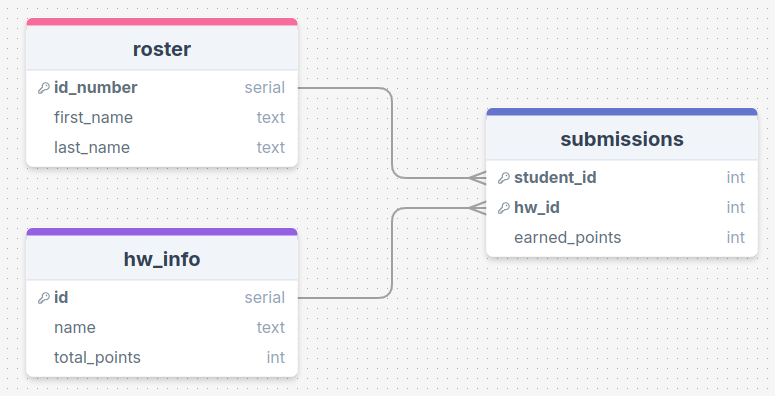{width=70%}
:::{.center .quip}
First names of students who have submitted any assignment?
:::
## Practice
{width=70%}
:::{.center .quip}
Student ID and name of the assignment for all perfect scores?
:::
## Practice
{width=70%}
:::{.center .quip}
Number of assignments with no submissions?
:::
## Practice
{width=70%}
:::{.center .quip}
All combinations of students and homework assignments?
:::
# Complicating Joins
## Multiple Join Conditionals
- You are not limited to just a single condition in your `ON` statement!
- You can chain multiple conditions together with `AND` or `OR`, just like you could with `WHERE`
- Just recall when comparing two rows that ALL the conditions must be true for the data to be included in the joined table
```pgsql
SELECT *
FROM table1
JOIN table2
ON table1.col1 = table2.col1
AND table1.col2 > table2.col2;
```
## Table Aliases
- Including long table names before each column name when referring to information from two different tables can get tedious
- You can define aliases for table names just like you can for column names!
- Syntax looks just like column aliases, using `AS`
- Can come immediately after you first reference a table name
- Usually after a `FROM` or `JOIN` statement
- In truth, the `AS` is optional, but it helps some with readability
```{.pgsql style='font-size:.9em'}
SELECT *
FROM tablename AS tn
JOIN tablename2 AS tn2
ON tn.col1 = tn2.col2;
```
## Multiple Joins
- Nothing stops you from including multiple joins in your query
- Each additional join links back to the current growing joined table
- This means a second join is treating the entire initial join as the "left" table
- Commonly, you'll just be joining back to the original table, so it won't be apparent
```pgsql
SELECT *
FROM tablename AS t1
JOIN tablename2 AS t2 ON t1.col1 = t2.col1
JOIN tablename3 AS t3 ON t1.col2 = t3.col1;
```
## More Practice
{width=70%}
:::{.center .quip}
First names of all individuals who are missing at least one assignment (no submission made)?
:::
## Self Joins
- You can actually join a table to itself!
- Why would you want to do this?
- Hierarchy data can frequently be explored in this fashion
- Comparisons between rows of a table
- You **need** to give unique aliases when doing this, or else you won't have a way to distinguish between which columns you want
## Joins as Venn Diagrams
- Sometimes it may help to think of different types of joins as Venn diagrams
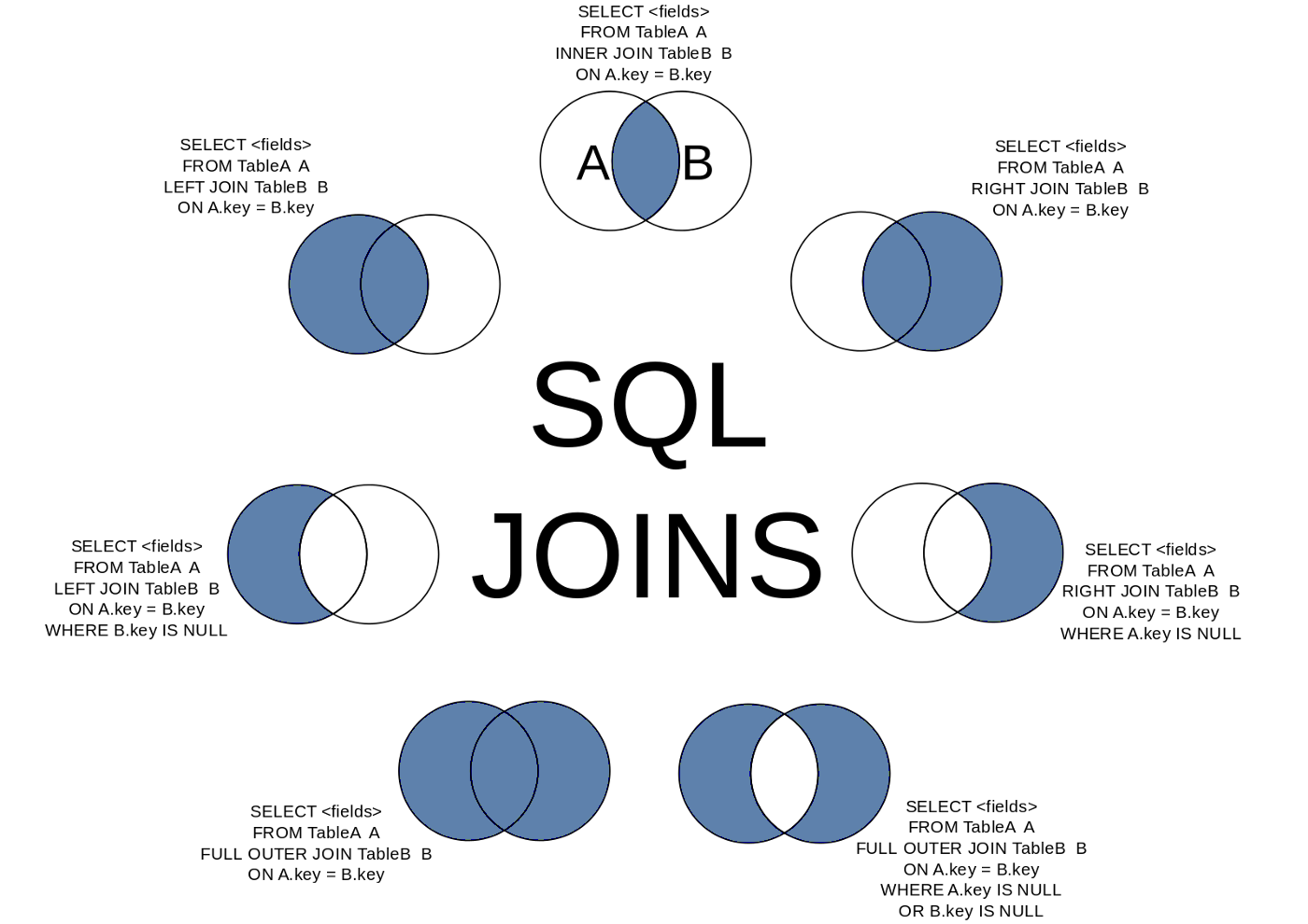{width=60%}