---
title: "Grouping JSON Model Indexes"
author: Jed Rembold
date: February 19, 2025
slideNumber: true
theme: nord_light
highlightjs-theme: nord
width: 1920
height: 1080
transition: slide
---
## Announcements
- Homework 5 due tonight!
- Homework 6 due next Wednesday
- **No class next week!**
- I'll be in Pittsburgh for SIGCSE
- Instead, next Wednesday you'll be sent the description and requirements of the midterm tutorial video assignment
- You'll have until the following Wednesday (March 5th) to submit a link to that upload
# Building a Model
## Data Modeling
- Data Modeling is the act of best deciding how to represent and store data such that it relates to the real world
- As much as possible, it is generally desirable to:
- ensure the model can easily help answer the types of questions you will want to ask
- operate at as low a level of granularity as possible
- remove redundancy
- ensure referential integrity
## Normalization
- First introduced by Edgar Codd in the early 1970s
- Codd outlined the following goals:
- to free the collection of relations from undesirable insertion, update, and deletion dependencies
- To reduce the need for restructuring the collection of relations as new types of data are introduced
- To make the relational model more informative to users
- To make the collection of relations neutral to what queries are being run on them
- To assist in these efforts, Codd introduced the idea of _normal forms_
## What is normal?
- Each normal form builds on those before
- The primary normal forms are:
Denormalized
: No normalization. Nested and redundant data is allowed
First normal form (1NF)
: Each column is unique and has a single value. The table has a unique primary key.
Second normal form (2NF)
: Partial dependencies are removed (only necessary if compound primary key)
Third normal form (3NF)
: Each table contains fields only relevant to its primary key, and has no transitive dependencies
## Denormalized
::::cols
:::col
- APIs will commonly give denormalized data, since they tend to return JSON type entries
- Consider the entry to the right about a particular order
:::
:::{.col style='flex-grow:2'}
```{.json style='max-height:1000px; font-size:.9em;'}
{ "OrderID": 100,
"OrderItems": [
{
"sku": 1,
"price": 10,
"quantity": 1,
"name": "Thingmajig"
},
{
"sku": 2,
"price": 25,
"quantity": 2,
"name": "Whatchamacalit"
}],
"CustomerID": 5,
"CustomerName": "Jed Rembold",
"OrderDate": "2022-11-09" }
```
:::
::::
## Initial Attempt
## 1st Normal Form
:::{style='font-size: .8em'}
| OrderID | Sku | Price | Quantity | ProductName | CustomerID | CustomerName | OrderDate |
|---------|-----|-------|----------|----------------|------------|--------------|------------|
| 100 | 1 | 50 | 1 | Thingmajig | 5 | Jed Rembold | 2022-11-09 |
| 100 | 2 | 25 | 2 | Whatchamacalit | 5 | Jed Rembold | 2022-11-09 |
:::
## 1st Normal Form (PK)
:::{style='font-size: .7em'}
| OrderID | ItemNum | Sku | Price | Quantity | ProductName | CustomerID | CustomerName | OrderDate |
|:--------:|:--------:|:---:|:-----:|:--------:|:---------------|:----------:|--------------|------------|
| 100 | 1 | 1 | 50 | 1 | Thingmajig | 5 | Jed Rembold | 2022-11-09 |
| 100 | 2 | 2 | 25 | 2 | Whatchamacalit | 5 | Jed Rembold | 2022-11-09 |
:::
## Evaluating 2NF
- To be in second normal form, there can be no partial dependencies, where columns depend on only one of the compound keys
- Here though the last 3 columns all depend only on OrderID
- Solution: Split to new tables!
## 2nd Normal Form
| OrderID | CustomerID | CustomerName | OrderDate |
|:--------:|:----------:|--------------|------------|
| 100 | 5 | Jed Rembold | 2022-11-09 |
| OrderID | ItemNum | Sku | Price | Quantity | ProductName |
|:--------:|:--------:|:---:|:-----:|:--------:|----------------|
| 100 | 1 | 1 | 50 | 1 | Thingmajig |
| 100 | 2 | 2 | 25 | 2 | Whatchamacalit |
## Evaluating 3NF
- The third normal form prohibits transitive dependencies, where a column depends on another (that depends on the primary key), instead of depending directly on the primary key
- Here we have 2! One in each table:
- `ProductName` depends on `Sku`
- `CustomerName` depends on `CustomerID`
- Solution? More tables!
## 3rd Normal Form
:::{style='font-size:.9em'}
| Sku | ProductName |
|:----:|----------------|
| 1 | Thingmajig |
| 2 | Whatchamacalit |
| CustomerID | CustomerName |
|:-----------:|--------------|
| 5 | Jed Rembold |
| OrderID | ItemNum | Sku | Price | Quantity |
|:--------:|:--------:|:---:|:-----:|:--------:|
| 100 | 1 | 1 | 50 | 1 |
| 100 | 2 | 2 | 25 | 2 |
| OrderID | CustomerID | OrderDate |
|:--------:|:----------:|------------|
| 100 | 5 | 2022-11-09 |
:::
## Visually
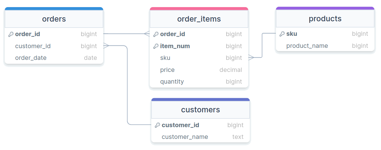{width=100%}
## Beyond
- Other normal forms exist (up to 6NF in the Boyce-Codd system)
- Most people only care about the first 3 to get data in a "normalized" state
- Unless you have specific performance reasons for wanting otherwise, you really should strive for normalized tables in your relational database, as they make maintaining, adding, updating, and adjusting your database and tables much easier
## Activity
:::smaller
- Think back to the Spotify modeling that we were playing around with last week
- Suppose you have the following information you need to store for each track:
| Info | Description |
|------------|----------------------------------------------|
| Track Name | The name of the track |
| Artists | Comma separated list of contributing artists |
| Album | The album this specific track appears on |
| Duration | The duration of the track in seconds |
| Genre | The general genre of the track |
| Track Num | The placement of this track on the album |
- Your task is to model this information into purely tables of 3NF
:::
## Activity Example Data
- Sometimes it helps to have some example data to look at:
:::smaller
| TName | Artists | Album | Duration | Genre | TNum |
|----------------------|-------------------|-----------------------------|----------|-------------|------|
| Don't Stop Believin' | Journey | Greatest Hits | 249 | Rock | 2 |
| Don't Stop Believin' | Journey | Escape | 251 | Rock | 1 |
| Fifteen | Taylor Swift | Fearless (Taylor's Version) | 294 | Country Pop | 2 |
| Under Pressure | Queen,David Bowie | Greatest Hits | 238 | Rock | 7 |
:::
# Indexing
## Consulting an Index
- Like in a book, an _index_ is a precomputed guide to help find things faster
- We can construct similar precomputed guides for certain columns in SQL to also help find things faster!
- There are several different types of indexes
- By default, the assigned index type is a B-Tree index in Postgres
- B-Tree stands for _balanced tree_ and work best for _orderable_ type data
- Index types like _Generalized Inverted Index_ (GIN) and _Generalized Search Tree_ (GiST) will be discussed later as they come up
- Different columns in the same table can be indexed with different methods
## Climbing a B-Tree
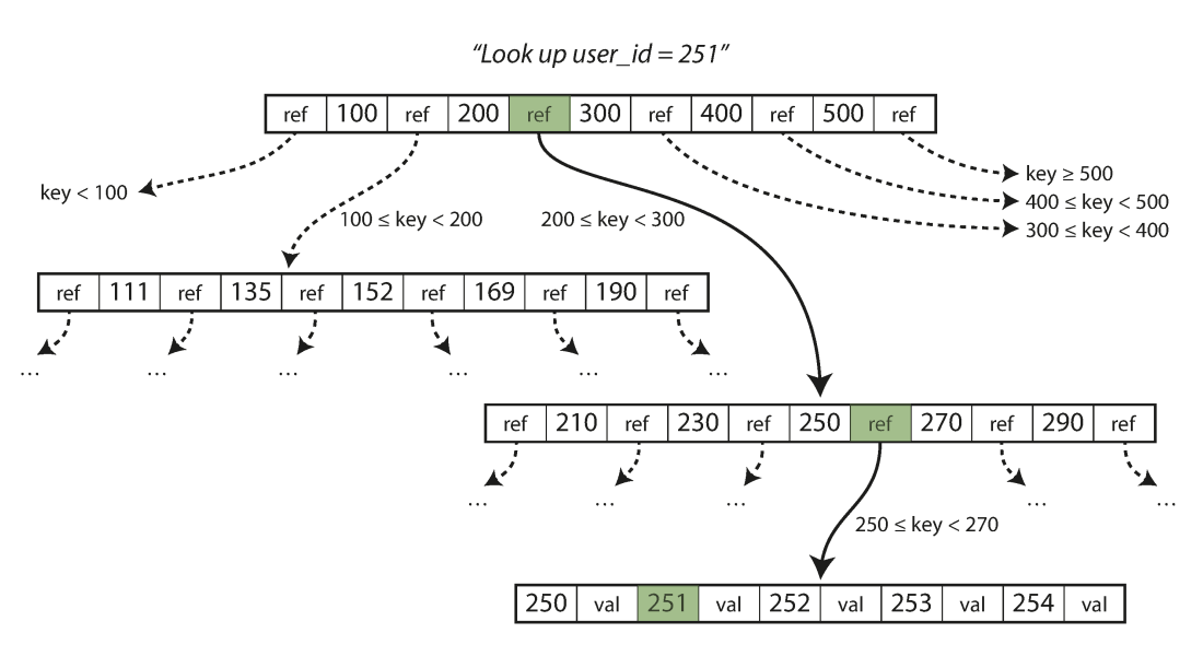{width=80%}
## Creating Indexes
- Postgres will automatically index any column that is a primary key or which has the `UNIQUE` constraint
- You can choose to set up indexes on other columns as well, but do so outside of the table creation
```{.pgsql style='font-size:1em'}
CREATE INDEX |||index name||| ON |||table name||| (|||column|||);
```
- If you decide you want to remove an index, you do so using the index name:
```{.pgsql style='font-size:1em'}
DROP INDEX |||index name|||;
```
## Benchmarking
- How can we objectively test this?
- Postgres has the `EXPLAIN` keyword to give you information about what the database is doing in the background
- Using `EXPLAIN ANALYZE` will also give you timing information about how long it took a query to run
- `EXPLAIN` always comes at the start of your query
```pgsql
EXPLAIN ANALYZE
SELECT * FROM |||table name|||
WHERE |||condition|||;
```
- Other SQL variants have their own versions, but most have some method of getting information back about execution time or what is being done under the hood
## Benchmarking Caveats
- `EXPLAIN ANALYZE` reports to you the time it took the server to process the query, not necessarily the time it took your client to finish getting and rendering the response!
- Especially for queries that return a huge number of rows, you might see a significant difference
- Indexes are optimized for certain types of operations. Just because you index a column doesn't mean that Postgres will **use** that index if you are doing an incompatible operation!
- Check more than just the timings from `EXPLAIN ANALYZE`
- See comments about Bitmaps and Heaps? Then the index was used.
- See comments about Parallel or Seq scans? Then the index was not used.
## Costs
- Indexes always have a cost associated with them, both in initial setup and in every time new data is added to the column
- Also, they are stored information, so they can also inflate your database size
- Consider indexing only those columns that receive the heaviest of use in filters or in joining
- You never need to worry about indexing primary keys or unique columns, as those are done automatically
- Indexing of _foreign keys_ though is not automatic, and might be a good idea for large datasets
- When in doubt, **benchmark** your queries before and after adding an index to see if you are really gaining much from it!
## Benchmarking Activity
- Most likely, you already (still) have the NYC Taxi Rides data on your computer
- Benchmark that data set under three different queries, for each getting a time both before creating an index and then after creating an index over the filtered column
- Select all the columns for the row where the ride id = 56789
- Select all the columns for the rows where the total amount charged was greater than $40
- Select all the columns for the rows where the total amount charged was greater than $10
- Enter your values into the shared spreadsheet [here](https://docs.google.com/spreadsheets/d/1WLhoEYzDR3I6LZqeZZ-FM0lmdiTKde_Ygwk1f5_sQRk/edit?usp=sharing) (Just choose an unused trial number)
# Break!
## Break Time!

# Grouping
## Birds of a Feather
- It is frequently the case that values in a particular table column all belong to a smaller subset of categories or options
- Think months of the year or political parties
- With current methods, if you want to compare some sort of aggregate between those categories or options, you need to do it in multiple queries:
:::::cols
::::col
```pgsql
SELECT AVG(age)
FROM voters
WHERE party = 'D'
```
::::
::::col
```pgsql
SELECT AVG(age)
FROM voters
WHERE party = 'R'
```
::::
:::::
- This rapidly becomes intractable if you want to compare across many categories
## The Fix
:::smaller
- SQL has one last fundamental trick up its sleeve with the `GROUP BY` command
- `GROUP BY` gathers together all rows with matching values from a particular column
- By itself, this is basically the same as running `DISTINCT` on a column
- Note that once you make a grouping, you can only select entire columns that are a part of the grouping
```pgsql
SELECT |||grouped column|||
FROM |||table name|||
GROUP BY |||grouped column|||;
```
- Can visualize as if many smaller tables were created, one for each grouping, which are then joined back together with each table contributing one row
:::
## Aggregating Groups
- Groups by themselves are not that useful, since we already had `DISTINCT`
- The prime use-case of `GROUP BY` is to be able to run aggregates across _all_ potential groups _simultaneously_ for comparison
```pgsql
SELECT
|||grouped column|||,
min(|||some other column|||),
avg(|||some other column|||)
FROM |||table name|||
GROUP BY |||grouped column|||;
```
- Causes any aggregate function to just aggregate over the smaller, group tables
## Group Example
Looking back at the cereal table, how can we answer:
- Which manufacturer sells the most sugar-laden cereal?
- What shelf has the most cereals placed on it? What about the greatest calorie average?
## MULTIPLE GROUPS
- Like with `DISTINCT` or `UNIQUE`, you can group by multiple columns
- Essentially splits the sub-tables into even smaller tables, one for each combination
```pgsql
SELECT
|||grouped col1|||,
|||grouped col2|||,
min(|||other col|||),
avg(|||other col|||)
FROM |||table|||
GROUP BY |||grouped col1|||, |||grouped col2|||
```
## HAVE or HAVE NOT
- You can not filter based on aggregates using `WHERE`
- `WHERE` actions happen before any aggregates can be computed
- If you want to filter your grouped results, you need to use `HAVING`
- `HAVING` filters take place **after** groups and aggregates have been computed
```pgsql
SELECT
|||grouped col|||
min(|||other col|||),
avg(|||other col|||)
FROM |||table|||
GROUP BY |||grouped col|||
HAVING min(|||other col|||) > 50;
```
## Server Ordering
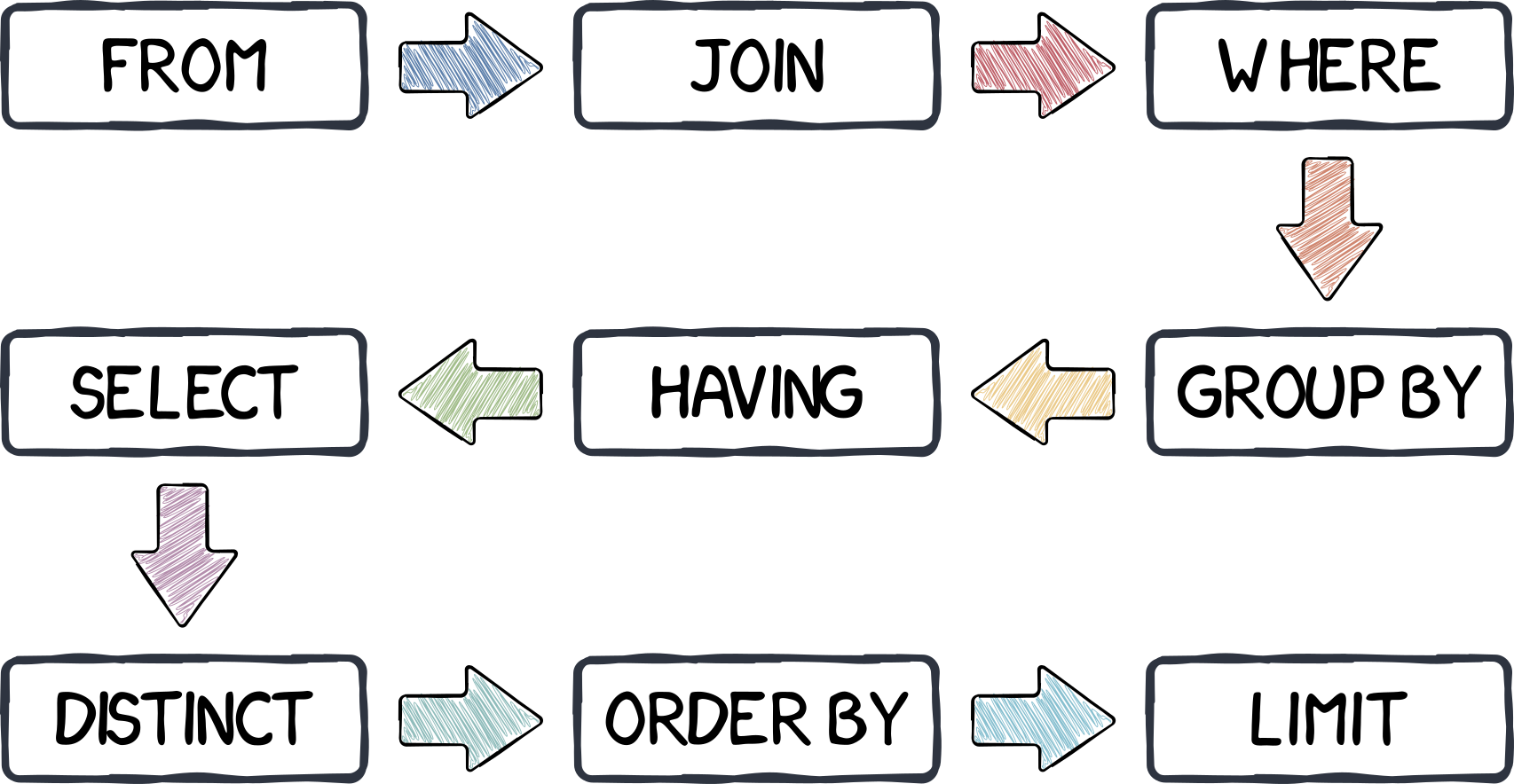{width=80%}
# Who's Son?
## JSON in Postgres
- One data type that we haven't discussed yet in Postgres is `json`
- Postgres actually support two `json` types:
- `json`: stores data as text
- Slower to process, but maintains whitespace and key orderings
- `jsonb`: stores data in a binary format
- Slightly slow to insert, but much faster to process
- Can have indexes defined
- In general, `jsonb` is probably preferable unless you really need what the base `json` type offers
## Populating JSON Tables
- JSON is frequently given with the outermost type being a list, and then each record inside separated by commas
- Postgres will **not** innately be able to import this type of document
- Instead, Postgres `COPY` works best when the JSON is a newline delimited JSON file (sometimes called jsonlines), where each new record is on a single line, and there is no surrounding `[]`
```pgsql
COPY |||table name|||
FROM |||your newline json file|||.json
```
- Want to follow along? A jsonlines file is [here](../activity_data/jsondemo.jsonlines)!
## JSON Selections
- You can drill down and select specific values from `json` or `jsonb` types using two different syntaxes:
- `raw_json -> 'key'/index` where:
- key is a string for key-value pairs
- index is an integer for arrays (0-based!)
- `raw_json['key'/index]` with the same conventions as above
- These can be "chained" to "drill down" to the desired info
```postgresql
raw_json -> 'siblings' -> 0 -> 'name'
```
- These selections return more `json`/`jsonb` objects! Convert as needed
- Using `->>` will instead return a `TEXT` type object
## JSON Existence
- Recall that JSON does not enforce a strict schema, so some entries may have keys or values that others are missing
- It can thus be useful to check for the existence of certain keys or values
- You can check if an entire chunk is contained within a block of JSON using `@>`:
```pgsql
raw_json @> |||sub-snippet of json|||
```
- You can also check if a key or value shows up in the **top level** of the JSON block using `?`:
```pgsql
raw_json ? |||top-level key|||
```
## JSON Indexes
- While you can create a default B-tree index for `jsonb` columns, they generally wouldn't be very useful
- Instead, we can use a different type of index called a _generalized inverted index_, or GIN
- This type of index works much better when the data is comprised of nested composite items (we'll see it again when we look at text searching)
- Just add `USING GIN` to your normal command to make an index
```pgsql
CREATE INDEX |||my index||| ON |||mytable||| USING GIN (|||colname|||);
```
# A Question of Timing
## Date-Time Reminders
- We have about 4 current date or time related data types
- Date time types:
- `DATE`: holds a single individual day
- `TIME`: holds a single individual time
- `TIMESTAMP` or variants with `TIMESTAMPTZ`: holds a combination of date and time, along with a potential time zone
- Interval types:
- `INTERVAL`: holds a duration of time
## Extracting Pieces
- Having all the information in one value is convenient, but sometimes you only need pieces
- The hour from the time, or the month from the date
- These can be particularly important with aggregates!
- Two methods to extract pieces of any datetime or interval type:
- SQL standard: `extract( part FROM |||datetime_value||| )`{.pgsql}
- Postgres specific: `date_part( |||part|||, |||datetime_value||| )`
- Both will return a `DOUBLE PRECISION` value of whatever part was requested
## Parts To Extract
- You have a wide variety of what you can extract
:::{style='font-size:.60em'}
::::::cols
::::col
| text | Description |
|--------------|-------------------------------------------------------------|
| century | What century the date is in. 1st century starts 0001-01-01[★]{.orange} |
| day | What day of the month |
| decade | The year divided by 10 |
| dow | The day of the week (0-6, starting with Sunday) |
| doy | The day of the year |
| epoch | Number of seconds since 1970-01-01 |
| hour | The current hour (0-23) |
| microseconds | The number of microseconds |
::::
::::col
| text | Description |
|---------------|--------------------------------------------------|
| milliseconds | The number of milliseconds |
| minute | The minute |
| month | The month (1-12) |
| quarter | What quarter of the year (1-4) |
| second | The number of seconds |
| timezone | The timezone offset in seconds |
| timezone_hour | The timezone offset in hours |
| week | What week of the year. ISO weeks start on Monday |
| year | The year |
::::
::::::
:::
:::{style='font-size:.5em'}
[★]{.orange} -- If you disagree with this, please write your complaint to: Pope, Cathedral Saint-Peter of Roma, Vatican.
:::
## Reversing it
:::{style='font-size:.9em'}
- Often times existing data sets have already separated out different aspects of the date or time
- Year, month, and day might be in different columns for example
- It can be useful to "stitch" these together into an actual datetime type for further use.
- Postgres gives you a handful of functions to do so:
- `make_date( |||year|||, |||month|||, |||day|||)`: Returns a new `DATE` type value
- `make_time( |||hour|||, |||minute|||, |||seconds||| )`: Returns a new `TIME` type value (with no timezone)
- `make_timestamptz(|||year|||,|||month|||,|||day|||,|||hour|||,|||minute|||,|||second|||,|||time zone|||)`: Returns a new `TIMESTAMPTZ` type value
- `make_timestamp` and `make_interval` also exist
:::
## Aging well
- Subtracting two `DATE` type values will give just an `INT` (in days)
- Subtracting two `TIMESTAMP` type values will give an `INTERVAL`, with the biggest "unit" in days
- Using Postgres's `age()` function can smooth over both and give units larger than days
- `age( datetime1, datetime2 )`: Subtracts datetime2 from datetime1
- This can **still** give you awkward interval units at times though, so also consider using `justify_interval( interval )`, which breaks intervals into divisions that don't exceed a categories max
- Hours would always be between 0 and 23 for instance, or months between 1 and 12
- Especially if you want to extract a particular part, this is highly recommended
## What time is it?
- Standard SQL also provides constants for grabbing the current system time and date
:::{style='font-size:.8em'}
| function | description |
|-----------------------------------|----------------------------------------------------|
| `current_date` | Returns the current date |
| `current_time` | Returns the current time with timezone |
| `localtime` | Returns the current time without timezone |
| `current_timestamp`[★]{.orange} | Returns the current date and time with timezone |
| `localtimestamp` | Returns the current date and time without timezone |
:::
[★]{.orange} -- Postgres also offers the shorter `now()` _function_ to do the same thing
## Time Zones
- Dealing with time zones can be a headache, and it is a very nice feature that Postgres can work with them smoothly
- By default, Postgres will _display_ any timestamp with a time zone with the time as you would measure it in your current system timezone
- What is your current system timezone?
- `SHOW timezone;`
- Getting general information about timezones:
- Getting abbreviations:
- `SELECT * FROM pg_timezone_abbrevs;`
- Getting full names:
- `SELECT * FROM pg_timezone_names;`
## Teleportation
- It can sometimes be useful to switch your "current" time zone
- Maybe it is easier to compare times to someone else living in that time zone
- Several methods to make the switch:
- Change your `postgressql.conf` file, which controls your Postgres server. Only recommended if you have permanently moved elsewhere and the database time zone has not updated appropriately.
- Set future queries in a single session to be from a new timezone:
`SET timezone TO time_zone_name_or_abbrv;`
- This will also adjust what values your `localtime` or `localtimestamp` report!
- Transform a single query to be reported in a different time zone:
```pgsql
SELECT |||datetime column||| AT TIME ZONE |||tz name or abbr|||
FROM |||table name|||;
```
## Activity
- Using the taxi rides dataset, see if you can:
- Compute the number of rides given each hour of the day
- Compute the average cost of rides over each day of the month
- Compute the median cost of rides over each day of the week
- Compute the average duration of each ride over each hour of the day