Lab 8: Exploring Complex Numbers
CS145: Images and Imagination, Spring 2010

 

Goals

• Gain the necessary background leading up to implementing fractals (Mandelbrot, Julia)
• Learn about and explore the behavior of complex numbers.
• Learn what a class is, and how to use classes (object oriented programming).
• Learn about rescaling and the map() function.
• Learn about iteration.

Resources and Readings

• Why Complex Numbers
• Wikipedia
• Wolfram MathWorld

Activities

1. Computing Complex Numbers by Hand: In class, we will go over the origin, definition, and operations of complex numbers. Once you are comfortable with the concepts, work through the following problems: Complex Number Problems (pdf).

   The solutions can be found here (pdf) but it is important that you try to do these without first looking at the solutions!

2. Computing Complex Numbers in Processing: Download and run the code complexClass.pde. We will go through it in class. Note, complex numbers are stored using a "Complex" Class. A Class is a description of a new data type. When we create (or instantiate) a variable of that type, it is called an object. You do not have to understand all of the syntax. Mostly what you should understand is how to create a Complex object and how to do various operations on the Complex object. The code in setup() illustrates how you would use this function to multiply two complex numbers.

   If you look at the functions in the Complex number class, you will see the function for cMult. Also note that the cAdd, cSub, and cDiv functions are commented out and not fully implemented. Following the pattern in cMult together with what you know about complex number operations, uncomment and complete the code for the cAdd, cSub, and cDiv functions. Test your code by using the problems you solved in the above Complex Number Problems. Note, you should be able to use the code to compute the solutions for all of the problems. This will both test the correctness of your cAdd, cSub, and cDiv functions, but will also give you practice using the syntax.

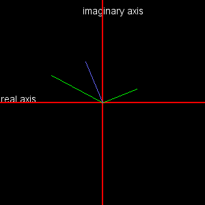
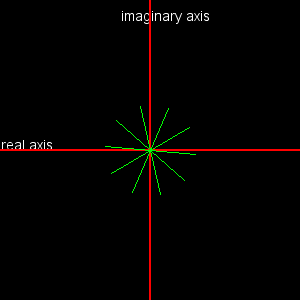
3. Plotting Complex numbers: To see the numbers plotted on the complex plane, create a new Processing sketch containing the code below. Also, copy your Complex class from the previous problem above and paste it at the bottom of this code. When you run the code, you will get the image below on the left. You only need to follow the code in drawComplex() (ignore the rest of the code). Try plotting other operations (e.g. mult, subtract).

   PFont font; void setup() { size(500,500); background(0); font = createFont("FFScala", 20); textFont(font); stroke(255); setUpCoordinates(); drawComplex(); } void drawComplex() { Complex c1 = new Complex(50,20); // create c1 Complex c2 = new Complex(-75,40); // create c2 Complex sum = Complex.cAdd(c1,c2); // sum c1 and c2 stroke(0,255,0); line(0,0,c1.real,c1.imag); // plot c1 line(0,0,c2.real,c2.imag); // plot c2 stroke(100,100,255); line(0,0,sum.real,sum.imag); // plot sum } // Flip y axis so up is positive. // Draw coordinate axes (real and imaginary). // Shift origin to center of window. void setUpCoordinates() { translate(width/2, height/2); // move origin to center text("real axis",-width/2,0); text("imaginary axis",-30,-height/2+20); scale(1,-1); // flip y axis so "positive" is up stroke(255,0,0); strokeWeight(2); line(-width/2,0,width/2,0); line(0,-height/2,0,height/2); stroke(255); strokeWeight(1); }

4. Iterating: Replace the drawComplex() function above with the following:

   void drawComplex() { stroke(0,255,0); Complex c = new Complex(34,-30); // create new complex number (34 - 30i) Complex m = Complex.polar2Cart(1.1, 30); // create a new complex number with // length 1.1 and angle 30 degrees for (int i = 0; i < 10; i ++) { c = Complex.cMult(c,m); line(0,0,c.real,c.imag); } }

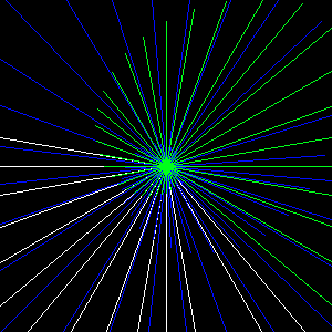
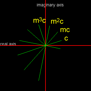
   The code starts with plotting a complex number c, and then plots m*c, m*m*c, etc, where m is a second complex number. This is an example of iteration - each time through the loop, the value of c is updated based on the previous value of c.

   Do you see why the complex numbers increase in length and angle, and why the angle rotates in a counter-clockwise direction?

   Modify the code (do you see how?) so that you get the following images:

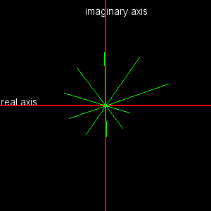   Here, the complex numbers do not change in length although the angle does change.	Here the complex numbers shrink in length.

5. Rescaling: So far, we have been drawing numbers to scale. That is, the line representing the complex number 10+0i will be 10 pixels long. Sometimes, we don't want to draw things to scale. For example, if you are an architect, your drawing plans for a house will not be the actual size of the house. Instead, it will be scaled (e.g. 10 feet = 1 inch) so that the drawing will fit on a normal piece of paper! Often, we want to do this as well. For example, when we implement the Mandelbrot set, we will be working in a region of the complex plane that extends from approximately from -2 to 2 units along the real axis and imaginary axes. It would not make sense to have 1 unit = 1 pixel because the image would not be visible. In this case, we need to increase the scale of the region so that it fits the entire window.

   For example, if want to represent the region from 0 to 1 (on both the real and imaginary axis), and if our window size is 100 pixels in height and width, then each pixel corresponds to .01 = (1/100) units or, we say that 1 pixel = .01 units in length in the complex plane. The origin may also be shifted. The question we need to figure out is, if we have a point in our complex region (e.g. .2+.7i), where will this go in our 100x100 pixel window? This all may sound confusing, but Processing makes it easy to do the rescaling by providing us with a map() function. Look in the online reference to see what the map() function does.

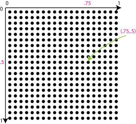
   For example, suppose we want to plot the region of the complex plane for 0 to 1 (real and imaginary) and that the window is 20x20 pixels as shown below. Where would the complex number .75 + .5i be placed in the window? To figure it out, we use the map function to determine the pixel associated with (.75,.5) as follows

   pixelX = map(.75, 0, 1, 0, 20); // gives 15 pixelY = map(.5, 0, 1, 0, 20); // gives 10 *************************************************** Syntax: map(value, low1, high1, low2, high2) Parameters value float: The incoming value to be converted low1 float: Lower bound of the value's current range high1 float: Upper bound of the value's current range low2 float: Lower bound of the value's target range high2 float: Upper bound of the value's target range

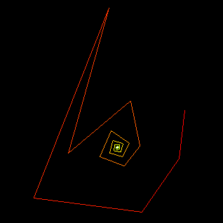
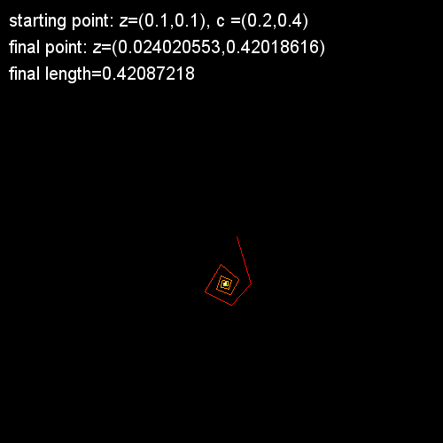
6. Orbits: Create a new Processing sketch and paste in the code below. You will also need to copy in the Complex number class from the previous part of the lab. In class, we will go over exactly what this code is doing. However, in a nutshell, it is generating an orbit generated by iterating on z = z² + c. The final point is identified by a white dot (depending on the initial point z, this may or may not be visible in the window. Below are some examples of images you get for different starting values.

   PFont font; Complex z = new Complex(0.63,.1); Complex c = new Complex(0.2,0.4); float px0, py0; void setup() { background(0); size(500,500); stroke(255); font = createFont("FFScala", 20); textFont(font); px0 = map(z.real,-1.5,1.5,0,width); py0 = map(z.imag, -1.5,1.5, 0, height); drawMe(); } void drawMe() { text("starting point: z=("+z.real+","+z.imag+"), c =("+c.real+","+c.imag+")", 10,30); int max = 100; colorMode(HSB, max); for (int i=0; i < max; i++) { stroke(i,max,max); // set color (HSB) z = Complex.cAdd(c,Complex.cMult(z,z)); // iterate z float pixelX = map(z.real,-1.5,1.5,0,width); // scale x float pixelY = map(z.imag, -1.5,1.5, 0, height); // scale y line(px0,py0,pixelX,pixelY); px0 = pixelX; py0 = pixelY; // Don't need this but it helps with debugging: println("z="+ z + " len = " + Complex.len(z) + " pixels: " + pixelX + "," + pixelY); } // This just draws the final value of z as a large white dot: stroke(0,0,max); // set color to white (HSB) strokeWeight(4); // set dotsize to be large point(px0,py0); // draw dot text("final point: z=("+z.real+","+z.imag+")", 10,60); text("final length="+ Complex.len(z), 10,90); save("orbit0.png"); } // add in your Complex class here.

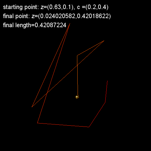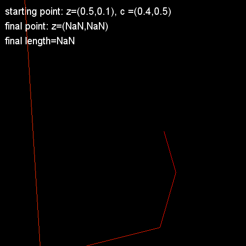7. Iteration Example - The Barnsley Fern: This example doesn't actually make use of complex numbers, but it is a good example of iteration and rescaling. The Barnsley fern is described here.

   Complete the code below based on the equations given at the web page. You need to add the remaining 3 parts of the if-else seequence and also fill in the appropriate values for the map function. Note, each of the 4 sets of equations (for each part of the if-else segments) is randomly executed some fraction of the time (Eqs1: 1%, Eqs2: 7%, Eqs3: 7%, and Eqs4: 85%). The way this is implemented is by generating a random number between 0 and 1000. The generated number will be below 100 approximately 1% of the time (do you see why?). You should get the image on the left.

   If you set the color to a different value for each if-else, you may be surprised at what you get.

   // sets the size and range of window: int windowWidth = 200; float xmin=-2.2, xmax = 2.7, ymin = 0, ymax = 10; float x=0, y=0; // starting x, y void setup() { size(windowWidth ,(int) (windowWidth*(ymax-ymin)/(xmax-xmin))); background(0); stroke(0,155,50); translate(0,height); scale(1,-1); // flip y axis so fern is upright for (int i = 0; i < 90000; i++) { iterate(); } save("fern.png"); } void iterate() { int r = (int) random(1000); if (r<10) { // selected 1% of the time x = 0; y = 0.16*y; } else if ( ) { // FINISH THIS - selected 7% of the time } else if ( ) { // FINISH THIS - selected 7% of the time } else if ( ) { // FINISH THIS - selected 85% of the time } // Scaling is based on window size and xmin,xmax,ymin,ymax float xscaled = map( ); // FILL THIS IN float yscaled = map( ); // FILL THIS IN point(xscaled,yscaled); }

Deliverables

Monday, April 5, before class:

The work in this lab is largely preparation for lab 9 so there is not a lot to turn in. Only Parts 6 and 7 have items to submit:

• Part 1: You no NOT need to turn in the written problems on complex numbers, however, it is expected that you know how to do this type of problem. If you have questions or need extra help, please see the instructor.
• Part 2: You no NOT need to turn in the Processing code, however, it is expected that you understand and practice using the syntax for creating and manipulating new Complex objects.
• Parts 3 & 4: You no NOT need to turn anything. This part of the lab is just intended to give you some intuition about Complex numbers. You should understand how complex numbers change (e.g. visually, in length, position, angle) when they are added, multiplied, etc..
• Part 5: You no NOT need to turn anything. We will use iteration and rescaling extensively in the next lab so it is important to understand them.
• Part 6: Turn in several sample images (no code needed!) of orbits (different from the examples given in the lab). Include at least one orbit that "blows-up", one that converges neatly, and one that is a bit chaotic looking but ultimately converges to a point. We will use orbits extensively in the next lab so it is important to understand them.
• Part 7: Turn in the code and sample image of your fern where you have used a different color for each part of the if-else. We will use iteration extensively in the next lab so it is important to understand it.